Meta 回归

Meta-regression 通过假设混合效应模型来实现。由于抽样误差和研究之间的异质性，观察到的研究偏离了真实的总体效应。

普通最小二乘法的加权版本

meta 回归使用一个或多个变量x来预测真实效应大小的差异。

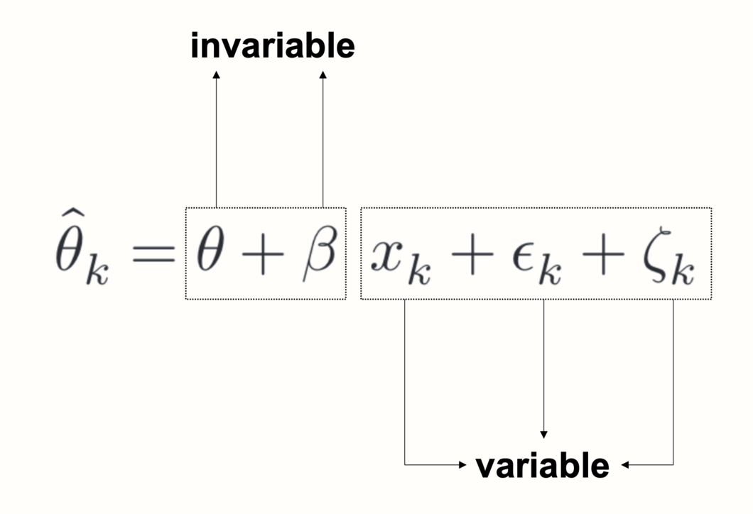
\[ \hat\theta_k = \theta + \beta x_{k} + \epsilon_k+\zeta_k \]

抽样误差$\epsilon_k$和研究间异质性 $\zeta_k$

固定效应（$\beta$）和随机效应（$\zeta_k$）

Meta回归模型

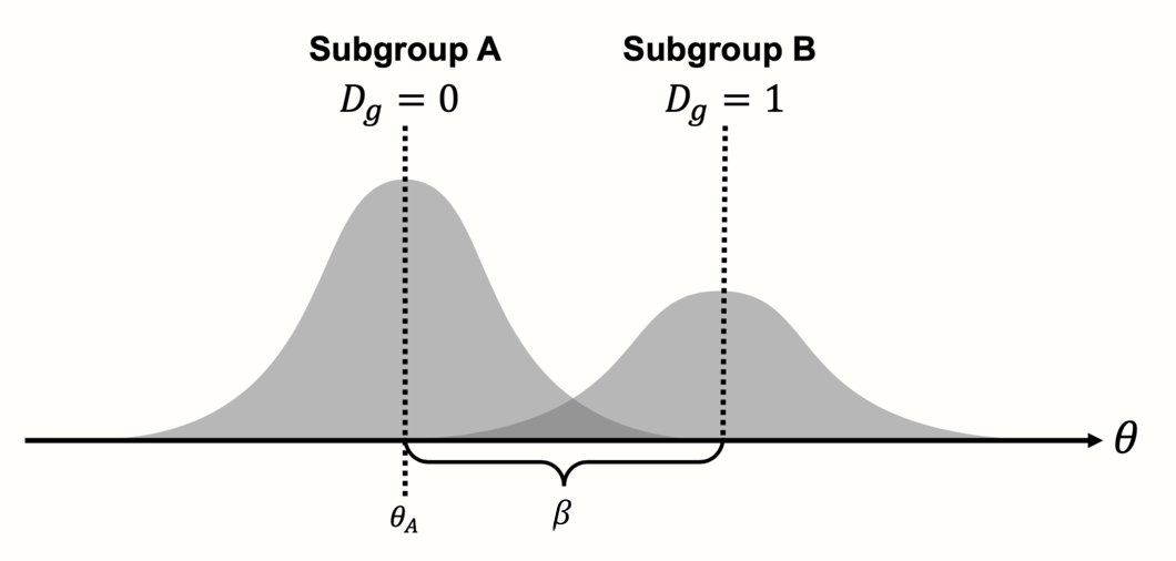
使用分类预测因子的meta回归

\[ \begin{equation} D_g=\begin{cases} 0: & \text{Subgroup A}\\ 1: & \text{Subgroup B.} \end{cases} \end{equation} \]

\[ \begin{equation} \hat\theta_k = \theta + \beta D_g +\epsilon_k+\zeta_k. \end{equation} \]

则

\[ \begin{equation} D_g=\begin{cases} 0: & \text{$\hat\theta_k = \theta_A + \epsilon_k+\zeta_k$}\\ 1: & \text{$\hat\theta_k = \theta_B + \theta_{\Delta} +\epsilon_k+\zeta_k$} \end{cases} \end{equation} \]

使用连续预测因子的meta回归

Show the code

library(meta)
m.gen <- metagen(TE = TE,
                 seTE = seTE,
                 studlab = Author,
                 data = dmetar::ThirdWave,
                 sm = "SMD",
                 fixed = FALSE,
                 random = TRUE,
                 method.tau = "REML",
                 method.random.ci = "HK",
                 prediction = T,
                 title = "Third Wave Psychotherapies")
summary(m.gen)

Review:     Third Wave Psychotherapies

                          SMD            95%-CI %W(random)
Call et al.            0.7091 [ 0.1979; 1.2203]        5.0
Cavanagh et al.        0.3549 [-0.0300; 0.7397]        6.3
DanitzOrsillo          1.7912 [ 1.1139; 2.4685]        3.8
de Vibe et al.         0.1825 [-0.0484; 0.4133]        7.9
Frazier et al.         0.4219 [ 0.1380; 0.7057]        7.3
Frogeli et al.         0.6300 [ 0.2458; 1.0142]        6.3
Gallego et al.         0.7249 [ 0.2846; 1.1652]        5.7
Hazlett-Stevens & Oren 0.5287 [ 0.1162; 0.9412]        6.0
Hintz et al.           0.2840 [-0.0453; 0.6133]        6.9
Kang et al.            1.2751 [ 0.6142; 1.9360]        3.9
Kuhlmann et al.        0.1036 [-0.2781; 0.4853]        6.3
Lever Taylor et al.    0.3884 [-0.0639; 0.8407]        5.6
Phang et al.           0.5407 [ 0.0619; 1.0196]        5.3
Rasanen et al.         0.4262 [-0.0794; 0.9317]        5.1
Ratanasiripong         0.5154 [-0.1731; 1.2039]        3.7
Shapiro et al.         1.4797 [ 0.8618; 2.0977]        4.2
Song & Lindquist       0.6126 [ 0.1683; 1.0569]        5.7
Warnecke et al.        0.6000 [ 0.1120; 1.0880]        5.2

Number of studies: k = 18

                             SMD            95%-CI    t  p-value
Random effects model (HK) 0.5771 [ 0.3782; 0.7760] 6.12 < 0.0001
Prediction interval              [-0.0542; 1.2084]              

Quantifying heterogeneity (with 95%-CIs):
 tau^2 = 0.0820 [0.0295; 0.3533]; tau = 0.2863 [0.1717; 0.5944]
 I^2 = 62.6% [37.9%; 77.5%]; H = 1.64 [1.27; 2.11]

Test of heterogeneity:
     Q d.f. p-value
 45.50   17  0.0002

Details of meta-analysis methods:
- Inverse variance method
- Restricted maximum-likelihood estimator for tau^2
- Q-Profile method for confidence interval of tau^2 and tau
- Calculation of I^2 based on Q
- Hartung-Knapp adjustment for random effects model (df = 17)
- Prediction interval based on t-distribution (df = 17)

Show the code

year <- c(2014, 1998, 2010, 1999, 2005, 2014, 
          2019, 2010, 1982, 2020, 1978, 2001,
          2018, 2002, 2009, 2011, 2011, 2013)

m.gen.reg <- metareg(m.gen, ~year)
m.gen.reg


Mixed-Effects Model (k = 18; tau^2 estimator: REML)

tau^2 (estimated amount of residual heterogeneity):     0.0188 (SE = 0.0226)
tau (square root of estimated tau^2 value):             0.1371
I^2 (residual heterogeneity / unaccounted variability): 29.26%
H^2 (unaccounted variability / sampling variability):   1.41
R^2 (amount of heterogeneity accounted for):            77.08%

Test for Residual Heterogeneity:
QE(df = 16) = 27.8273, p-val = 0.0332

Test of Moderators (coefficient 2):
F(df1 = 1, df2 = 16) = 9.3755, p-val = 0.0075

Model Results:

         estimate       se     tval  df    pval     ci.lb     ci.ub     
intrcpt  -36.1546  11.9800  -3.0179  16  0.0082  -61.5510  -10.7582  ** 
year       0.0183   0.0060   3.0619  16  0.0075    0.0056    0.0310  ** 

---
Signif. codes:  0 '***' 0.001 '**' 0.01 '*' 0.05 '.' 0.1 ' ' 1

$\hat\tau^2_{\text{unexplained}}=$ 0.0188

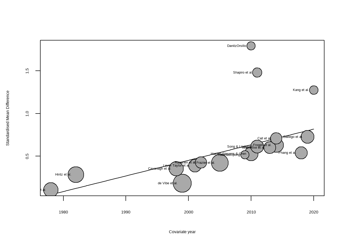
$R^2_*$ =77.08% 意味着真实效应大小的 77% 的差异可以用出版年份来解释，这是一个相当大的值。

Show the code

bubble(m.gen.reg, studlab = TRUE)

Show the code

# 通过meta回归进行亚组分析
metareg(m.gen, RiskOfBias)


Mixed-Effects Model (k = 18; tau^2 estimator: REML)

tau^2 (estimated amount of residual heterogeneity):     0.0691 (SE = 0.0424)
tau (square root of estimated tau^2 value):             0.2630
I^2 (residual heterogeneity / unaccounted variability): 60.58%
H^2 (unaccounted variability / sampling variability):   2.54
R^2 (amount of heterogeneity accounted for):            15.66%

Test for Residual Heterogeneity:
QE(df = 16) = 39.3084, p-val = 0.0010

Test of Moderators (coefficient 2):
F(df1 = 1, df2 = 16) = 2.5066, p-val = 0.1329

Model Results:

               estimate      se     tval  df    pval    ci.lb   ci.ub      
intrcpt          0.7691  0.1537   5.0022  16  0.0001   0.4431  1.0950  *** 
RiskOfBiaslow   -0.2992  0.1890  -1.5832  16  0.1329  -0.6999  0.1014      

---
Signif. codes:  0 '***' 0.001 '**' 0.01 '*' 0.05 '.' 0.1 ' ' 1

RiskOfBiaslow 效应大小 g = 0.7691-0.2992 ≈0.4699

多元回归

\[ \begin{equation} \hat \theta_k = \theta + \beta_1x_{1k} + ... + \beta_nx_{nk} + \epsilon_k + \zeta_k \tag{multiple-metareg} \end{equation} \]

Show the code

library(metafor)
library(tidyverse)
library(dmetar)
data(MVRegressionData)
glimpse(MVRegressionData)

Rows: 36
Columns: 6
$ yi         <dbl> 0.09437543, 0.09981923, 0.16931607, 0.17511107, 0.27301641,…
$ sei        <dbl> 0.1959031, 0.1918510, 0.1193179, 0.1161592, 0.1646946, 0.17…
$ reputation <dbl> -11, 0, -11, 4, -10, -9, -8, -8, -8, 0, -5, -5, -4, -4, -3,…
$ quality    <dbl> 6, 9, 5, 9, 2, 10, 6, 3, 10, 3, 1, 5, 10, 2, 1, 2, 4, 1, 8,…
$ pubyear    <dbl> -0.85475360, -0.75277184, -0.66048349, -0.56304843, -0.4308…
$ continent  <fct> 1, 0, 1, 0, 1, 0, 0, 0, 0, 0, 0, 1, 0, 0, 0, 0, 0, 0, 0, 1,…

多重共线性

Show the code

MVRegressionData[,c("reputation", "quality", "pubyear")] %>% 
    cor()

           reputation    quality    pubyear
reputation  1.0000000  0.3015694  0.3346594
quality     0.3015694  1.0000000 -0.1551123
pubyear     0.3346594 -0.1551123  1.0000000

Show the code

m.qual <- rma(yi = yi,
              sei = sei,
              data = MVRegressionData,
              method = "ML",
              mods = ~ quality,
              test = "knha")

m.qual


Mixed-Effects Model (k = 36; tau^2 estimator: ML)

tau^2 (estimated amount of residual heterogeneity):     0.0667 (SE = 0.0275)
tau (square root of estimated tau^2 value):             0.2583
I^2 (residual heterogeneity / unaccounted variability): 60.04%
H^2 (unaccounted variability / sampling variability):   2.50
R^2 (amount of heterogeneity accounted for):            7.37%

Test for Residual Heterogeneity:
QE(df = 34) = 88.6130, p-val < .0001

Test of Moderators (coefficient 2):
F(df1 = 1, df2 = 34) = 3.5330, p-val = 0.0688

Model Results:

         estimate      se    tval  df    pval    ci.lb   ci.ub    
intrcpt    0.3429  0.1354  2.5318  34  0.0161   0.0677  0.6181  * 
quality    0.0356  0.0189  1.8796  34  0.0688  -0.0029  0.0740  . 

---
Signif. codes:  0 '***' 0.001 '**' 0.01 '*' 0.05 '.' 0.1 ' ' 1

Show the code

m.qual.rep <- rma(yi = yi, 
                  sei = sei, 
                  data = MVRegressionData, 
                  method = "ML", 
                  mods = ~ quality + reputation, 
                  test = "knha")

m.qual.rep


Mixed-Effects Model (k = 36; tau^2 estimator: ML)

tau^2 (estimated amount of residual heterogeneity):     0.0238 (SE = 0.0161)
tau (square root of estimated tau^2 value):             0.1543
I^2 (residual heterogeneity / unaccounted variability): 34.62%
H^2 (unaccounted variability / sampling variability):   1.53
R^2 (amount of heterogeneity accounted for):            66.95%

Test for Residual Heterogeneity:
QE(df = 33) = 58.3042, p-val = 0.0042

Test of Moderators (coefficients 2:3):
F(df1 = 2, df2 = 33) = 12.2476, p-val = 0.0001

Model Results:

            estimate      se    tval  df    pval    ci.lb   ci.ub      
intrcpt       0.5005  0.1090  4.5927  33  <.0001   0.2788  0.7222  *** 
quality       0.0110  0.0151  0.7312  33  0.4698  -0.0197  0.0417      
reputation    0.0343  0.0075  4.5435  33  <.0001   0.0189  0.0496  *** 

---
Signif. codes:  0 '***' 0.001 '**' 0.01 '*' 0.05 '.' 0.1 ' ' 1

Show the code

anova(m.qual, m.qual.rep)


        df     AIC     BIC    AICc   logLik     LRT   pval      QE  tau^2 
Full     4 19.4816 25.8157 20.7720  -5.7408                58.3042 0.0238 
Reduced  3 36.9808 41.7314 37.7308 -15.4904 19.4992 <.0001 88.6130 0.0667 
             R^2 
Full             
Reduced 64.3197%

anova LRT X2= 19.4992 ,p<0.001

交互效应

Show the code

# Add factor labels to 'continent'
# 0 = Europe
# 1 = North America
levels(MVRegressionData$continent) = c("Europe", "North America")

# Fit the meta-regression model
m.qual.rep.int <- rma(yi = yi, 
                      sei = sei, 
                      data = MVRegressionData, 
                      method = "REML", 
                      mods = ~ pubyear * continent, 
                      test = "knha")

m.qual.rep.int


Mixed-Effects Model (k = 36; tau^2 estimator: REML)

tau^2 (estimated amount of residual heterogeneity):     0 (SE = 0.0098)
tau (square root of estimated tau^2 value):             0
I^2 (residual heterogeneity / unaccounted variability): 0.00%
H^2 (unaccounted variability / sampling variability):   1.00
R^2 (amount of heterogeneity accounted for):            100.00%

Test for Residual Heterogeneity:
QE(df = 32) = 24.8408, p-val = 0.8124

Test of Moderators (coefficients 2:4):
F(df1 = 3, df2 = 32) = 28.7778, p-val < .0001

Model Results:

                                estimate      se    tval  df    pval    ci.lb 
intrcpt                           0.3892  0.0421  9.2472  32  <.0001   0.3035 
pubyear                           0.1683  0.0834  2.0184  32  0.0520  -0.0015 
continentNorth America            0.3986  0.0658  6.0539  32  <.0001   0.2645 
pubyear:continentNorth America    0.6323  0.1271  4.9754  32  <.0001   0.3734 
                                 ci.ub      
intrcpt                         0.4750  *** 
pubyear                         0.3380    . 
continentNorth America          0.5327  *** 
pubyear:continentNorth America  0.8911  *** 

---
Signif. codes:  0 '***' 0.001 '**' 0.01 '*' 0.05 '.' 0.1 ' ' 1

过拟合

$R^2_*$ = 100% ，在实践中，几乎不会解释数据中的所有异质性——事实上，如果在现实生活中的数据中找到这样的结果，这可能是模型过度拟合了。

排列测试

Show the code

permutest(m.qual.rep)

Running 1000 iterations for an approximate permutation test.


Test of Moderators (coefficients 2:3):¹
F(df1 = 2, df2 = 33) = 12.2476, p-val = 0.0010

Model Results:

            estimate      se    tval  df    pval¹    ci.lb   ci.ub      
intrcpt       0.5005  0.1090  4.5927  33  0.1980    0.2788  0.7222      
quality       0.0110  0.0151  0.7312  33  0.4090   -0.0197  0.0417      
reputation    0.0343  0.0075  4.5435  33  0.0010    0.0189  0.0496  *** 

---
Signif. codes:  0 '***' 0.001 '**' 0.01 '*' 0.05 '.' 0.1 ' ' 1

1) p-values based on permutation testing

多模型推理

Show the code

multimodel.inference(TE = "yi", 
                     seTE = "sei",
                     data = MVRegressionData,
                     predictors = c("pubyear", "quality", 
                                    "reputation", "continent"),
                     interaction = FALSE)


  |                                                                            
  |                                                                      |   0%
  |                                                                            
  |====                                                                  |   6%
  |                                                                            
  |=========                                                             |  12%
  |                                                                            
  |=============                                                         |  19%
  |                                                                            
  |==================                                                    |  25%
  |                                                                            
  |======================                                                |  31%
  |                                                                            
  |==========================                                            |  38%
  |                                                                            
  |===============================                                       |  44%
  |                                                                            
  |===================================                                   |  50%
  |                                                                            
  |=======================================                               |  56%
  |                                                                            
  |============================================                          |  62%
  |                                                                            
  |================================================                      |  69%
  |                                                                            
  |====================================================                  |  75%
  |                                                                            
  |=========================================================             |  81%
  |                                                                            
  |=============================================================         |  88%
  |                                                                            
  |==================================================================    |  94%



Multimodel Inference: Final Results
--------------------------

 - Number of fitted models: 16
 - Full formula: ~ pubyear + quality + reputation + continent
 - Coefficient significance test: knha
 - Interactions modeled: no
 - Evaluation criterion: AICc 


Best 5 Models
--------------------------


Global model call: metafor::rma(yi = TE, sei = seTE, mods = form, data = glm.data, 
    method = method, test = test)
---
Model selection table 
   (Intrc) cntnn  pubyr   qulty   rpttn df logLik AICc delta weight
12       +     + 0.3533         0.02160  5  2.981  6.0  0.00  0.536
16       +     + 0.4028 0.02210 0.01754  6  4.071  6.8  0.72  0.375
8        +     + 0.4948 0.03574          5  0.646 10.7  4.67  0.052
11       +       0.2957         0.02725  4 -1.750 12.8  6.75  0.018
15       +       0.3547 0.02666 0.02296  5 -0.395 12.8  6.75  0.018
Models ranked by AICc(x) 


Multimodel Inference Coefficients
--------------------------

                         Estimate  Std. Error   z value  Pr(>|z|)
intrcpt                0.38614661 0.106983583 3.6094006 0.0003069
continentNorth America 0.24743836 0.083113174 2.9771256 0.0029096
pubyear                0.37816796 0.083045572 4.5537402 0.0000053
reputation             0.01899347 0.007420427 2.5596198 0.0104787
quality                0.01060060 0.014321158 0.7402055 0.4591753


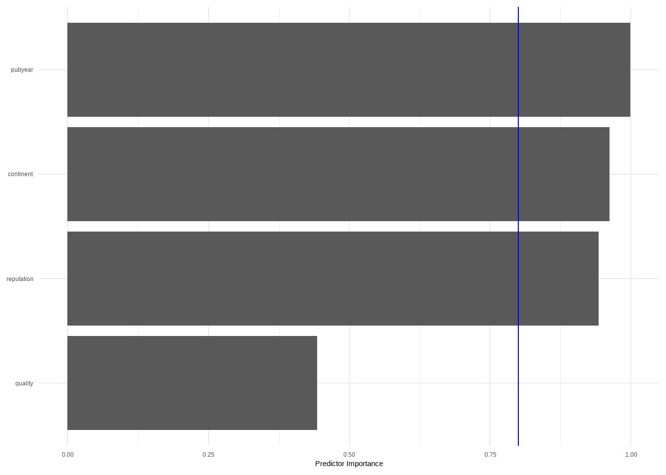
Predictor Importance
--------------------------

       model importance
1    pubyear  0.9988339
2  continent  0.9621839
3 reputation  0.9428750
4    quality  0.4432826