1 ggplot2 Graphics

ggplot2: Elegant Graphics for Data Analysis (3e)

gg 为 grammar of graphics 的缩写。

ggplot(data = ,mapping = aes(x,y,…))

创建一个基础图形对象gg,空白图层 + 数据集 + 美学映射。

1.1 Data

Code
library(tidyverse)
#> Warning: package 'purrr' was built under R version 4.5.2
#> Warning: package 'stringr' was built under R version 4.5.2
#> Warning: package 'forcats' was built under R version 4.5.2
#> ── Attaching core tidyverse packages ──────────────────────── tidyverse 2.0.0 ──
#> ✔ dplyr     1.1.4     ✔ readr     2.1.6
#> ✔ forcats   1.0.1     ✔ stringr   1.6.0
#> ✔ ggplot2   4.0.1     ✔ tibble    3.3.0
#> ✔ lubridate 1.9.4     ✔ tidyr     1.3.1
#> ✔ purrr     1.2.0     
#> ── Conflicts ────────────────────────────────────────── tidyverse_conflicts() ──
#> ✖ dplyr::filter() masks stats::filter()
#> ✖ dplyr::lag()    masks stats::lag()
#> ℹ Use the conflicted package (<http://conflicted.r-lib.org/>) to force all conflicts to become errors
library(patchwork)
#> Warning: package 'patchwork' was built under R version 4.5.2
df <- tibble(
    index = 1:26,
    pch = 0:25,
    type = c( rep("hollow_color",15),rep("soild_color",6),rep("fill_color",5)),
    height = rep(c(1,2,3), times = c(15,6,5)),
    
)

1.2 Aesthetics mapping

mapping=aes(x,y,z,..,color,fill,shape,size,group,linewidth,linetype,alpha,...)

Code
ggplot(data = df,
       mapping = aes(x = index, y = pch ))

1.3 Geometry

Code
df <- data.frame(
  x = c(3, 1, 5), 
  y = c(2, 4, 6), 
  label = c("a","b","c")
)

p <- ggplot(df, aes(x, y, label = label)) + 
  labs(x = NULL, y = NULL) + # Hide axis label
  theme(plot.title = element_text(size = 12)) # Shrink plot title

(p + geom_point() + ggtitle("point") +
        p + geom_text() + ggtitle("text") +
        p + geom_bar(stat = "identity") + ggtitle("bar") )/
(p + geom_tile() + ggtitle("tile") +
     p + geom_raster() + ggtitle("raster")+
     p + geom_line() + ggtitle("line")) /
(p + geom_area() + ggtitle("area") +
    p + geom_path() + ggtitle("path") +
    p + geom_polygon() + ggtitle("polygon"))

1.3.1 X=连续型变量

1.3.1.1 geom_point

Code
ggplot(data = mpg) + 
    geom_point(mapping = aes(x=displ,y=hwy),
               stat = "identity",position = "identity")

Code
ggplot(mpg, aes(displ,hwy)) +
    geom_point() |
    
    ggplot(mpg, aes(displ,hwy)) +
    geom_point(aes(size = displ/10)) + 
    scale_size_area(name="displ/10")

1.3.1.2 geom_line

Code
economics |> head()
#> # A tibble: 6 × 6
#>   date         pce    pop psavert uempmed unemploy
#>   <date>     <dbl>  <dbl>   <dbl>   <dbl>    <dbl>
#> 1 1967-07-01  507. 198712    12.6     4.5     2944
#> 2 1967-08-01  510. 198911    12.6     4.7     2945
#> 3 1967-09-01  516. 199113    11.9     4.6     2958
#> 4 1967-10-01  512. 199311    12.9     4.9     3143
#> 5 1967-11-01  517. 199498    12.8     4.7     3066
#> 6 1967-12-01  525. 199657    11.8     4.8     3018

ggplot(economics,aes(date,pop))+
    geom_line()+
    scale_x_date()

1.3.1.3 geom_smooth

Code
q <- ggplot(mpg, aes(displ, hwy)) +
    geom_point()

q+geom_smooth(method = "loess",span = 0.2,se=T) # loess 平滑局部回归   small n
#> `geom_smooth()` using formula = 'y ~ x'

Code
                                   #span 0非常摆动,1不那么摆动

q+ geom_smooth(span = 1)  #不很摆动
#> `geom_smooth()` using method = 'loess' and formula = 'y ~ x'

Code

library(MASS)
#> 
#> Attaching package: 'MASS'
#> 
#> The following object is masked from 'package:patchwork':
#> 
#>     area
#> 
#> The following object is masked from 'package:dplyr':
#> 
#>     select
q+geom_smooth(method = "rlm")   # robust linear model  稳健线性模型
#> `geom_smooth()` using formula = 'y ~ x'

Code

library(mgcv)
#> Warning: package 'mgcv' was built under R version 4.5.2
#> Loading required package: nlme
#> 
#> Attaching package: 'nlme'
#> 
#> The following object is masked from 'package:dplyr':
#> 
#>     collapse
#> 
#> This is mgcv 1.9-4. For overview type '?mgcv'.
q+ geom_smooth(method = "gam", formula = y ~ s(x)) # gam 广义相加模型   n>1000

Code
binomial_smooth <- function(...) {
  geom_smooth(method = "glm", method.args = list(family = "binomial"), ...)
}


ggplot(rpart::kyphosis,aes(Age,as.numeric(Kyphosis)-1))+
    geom_point()+
    binomial_smooth()
#> `geom_smooth()` using formula = 'y ~ x'

1.3.1.4 geom_histogram

Code
ggplot(mpg, aes(hwy)) + geom_histogram(binwidth = 2.5)

Code


ggplot(mpg, aes(hwy)) +
  geom_histogram(binwidth = 1) |
ggplot(mpg, aes(hwy)) +
  geom_histogram(aes(weight = displ), binwidth = 1) # 加权

Code

ggplot(data = mpg) + 
    geom_histogram(aes(x=displ,y=after_stat(density)),
                   stat = "bin",position = "stack",
                   binwidth = 0.5
                   ) +
    scale_y_continuous(labels=scales::percent) +
    geom_density(aes(x=displ,y=after_stat(density)),
                 color="red", linewidth=1)

1.3.1.5 geom_bin2d()

Code
smaller <- diamonds |> 
  dplyr::filter(carat < 3)
ggplot(smaller, aes(x = carat, y = price)) +
  geom_bin2d()
#> `stat_bin2d()` using `bins = 30`. Pick better value `binwidth`.

Code

# install.packages("hexbin")
ggplot(smaller, aes(x = carat, y = price)) +
  geom_hex()

1.3.1.6 geom_freqpoly

Code
ggplot(mpg, aes(hwy)) + 
  geom_freqpoly(binwidth = 2.5)

1.3.1.7 geom_density

Code

p <- ggplot(data = mpg)
p + geom_density(aes(displ,fill=drv),
                 stat = "density",position = "identity",
                 alpha=0.3
                 )+
    scale_y_continuous(labels = scales::percent)+
    labs(fill="图例名")+
    theme(legend.position = "top")

1.3.1.8 geom_rug

y→sides="r","l"

x→sides="b","t"

Code
p + geom_rug(aes(x=displ,y=hwy),
           sides = "br",color="brown")

1.3.1.9 geom_jitter

Code
p + geom_jitter(mapping = aes(x=displ,y=hwy),
               stat = "identity",position = "jitter")

1.3.2 X=离散型变量

1.3.2.1 geom_bar

Code
ggplot(data = mpg) + 
    geom_bar(mapping = aes(x=factor(cyl),fill=drv),
             stat = "count",position = "stack") |
ggplot(data = mpg) + 
    geom_bar(mapping = aes(x=factor(cyl),fill=drv),
             position = "dodge")

Code


ggplot(data = mpg) + 
    geom_col(mapping = aes(x=factor(cyl),y=hwy,fill=drv),
             position = "stack") |

ggplot(data = mpg) + 
    geom_col(mapping = aes(x=factor(cyl),y=hwy,fill=drv),
             position = "fill")+
    scale_y_continuous(labels = scales::label_percent())

有序条形图

Code
ggplot(mpg, aes(x = fct_infreq(class))) +  #降序条形图
  geom_bar()

1.3.2.2 geom_errorbar

  • geom_errorbarh

  • geom_linerange

  • geom_crossbar

  • geom_pointrange

Code
y <- c(18, 11, 16)
df <- data.frame(x = 1:3, y = y, se = c(1.2, 0.5, 1.0))

base <- ggplot(df, aes(x, y, ymin = y - se, ymax = y + se))
(base + geom_errorbar()|
base + geom_linerange()|
base + geom_ribbon())/
(base + geom_crossbar()|
base + geom_pointrange()|
base + geom_smooth(stat = "identity"))

Code
read_csv("data/g.csv") |> 
    summarise(
        mean=mean(liverweight),
        sd=sd(liverweight),
        .by=treatment
  ) |> 
    ggplot(aes(treatment,mean,fill=treatment))+
    geom_bar(stat = "identity")+
    geom_errorbar(aes(ymin=mean-sd,ymax=mean+sd),width=.2)
#> Rows: 20 Columns: 2
#> ── Column specification ────────────────────────────────────────────────────────
#> Delimiter: ","
#> chr (1): treatment
#> dbl (1): liverweight
#> 
#> ℹ Use `spec()` to retrieve the full column specification for this data.
#> ℹ Specify the column types or set `show_col_types = FALSE` to quiet this message.

1.3.2.3 geom_dotplot

Code
ggplot(mpg)+geom_dotplot(mapping = aes(x=drv,y=hwy),
                 position = "identity",
                 stackdir = "center",binaxis = 'y',# stacking along y axis
                 fill="red",binwidth = 0.7)

1.3.2.4 geom_boxplot

Code
ggplot(mpg) + geom_boxplot(mapping = aes(x=drv,y=hwy),
             stat = "boxplot",position = "dodge",
             notch=TRUE, varwidth=TRUE,
             width=0.1,fill="green"
            )+
    geom_violin(aes(x=drv,y=hwy),alpha=0.2)

1.3.2.5 geom_violin

Code
ggplot(mpg) + geom_violin(mapping = aes(x=drv,y=hwy),
             stat = "ydensity",position = "dodge")

1.3.2.6 geom_tile

Code
# 设置随机数种子以确保结果的可重复性  
set.seed(10)  
  
# 生成随机数据集  
mydata <- tibble(  
  year = 2000:2024,  
  lung = runif(25),  
  liver = runif(25), 
  bone = runif(25),  
  luk = runif(25),  
  eso = runif(25),  
  gas = runif(25),   
  eye = runif(25),  
  brain = runif(25),  
  pan = runif(25),  
  kidney = runif(25),  
  breast= runif(25),  
)  |> pivot_longer(cols = -1,
                   names_to = "cancer",
                   values_to = "morbidity")

ggplot(mydata, aes(year, cancer)) +  
  geom_tile(aes(fill =morbidity)) +  
  scale_fill_gradient(low = "white", high = "red")

1.4 Statistical transformations

stat_bin():geom_bar(),geom_freqpoly(),geom_histogram()

stat_bin2d():geom_bin2d()

stat_bindot():geom_dotplot()

stat_binhex():geom_hex()

stat_boxplot():geom_boxplot()

stat_contour():geom_contour()

stat_quantile():geom_quantile()

stat_smooth():geom_smooth()

stat_sum():geom_count()

stat_ecdf():计算经验累积分布图。

stat_function():根据 x 值的函数计算 y 值。

stat_summary():将 Y 值汇总到不同的 X 值。

Code
mtcars |> 
    ggplot(aes(x = factor(am) , y= mpg))+
    stat_summary(geom = "bar",fun = mean)

Code
ggplot(diamonds) + 
  stat_summary(
    aes(x = cut, y = depth),
    geom = "errorbar",
    fun.min = min,
    fun.max = max,
    fun = mean
  )

Code

ggplot(mpg, aes(trans, cty)) + 
    geom_point() + 
    stat_summary(geom = "point", fun = "mean", colour = "red", size = 4)

stat_summary2d() :汇总分箱值。

stat_summary_hex()

stat_qq():对分位数-分位数图执行计算。

stat_spoke():将角度和半径转换为位置。

stat_unique():删除重复的行。

1.5 Position adjustments

1.5.1 条偏移

Code
ggplot(mpg, aes(x = drv, fill = class)) + 
  geom_bar(alpha = 1/5, position = "identity")|

ggplot(mpg, aes(x = drv, color = class)) + 
  geom_bar(fill = NA, position = "identity")

Code

ggplot(mpg, aes(x = drv, fill = class)) + 
  geom_bar(position = "fill")|

ggplot(mpg, aes(x = drv, fill = class)) + 
  geom_bar(position = "dodge")

1.5.2 点偏移

position_nudge():按固定偏移量移动点。

position_jitter():为每个位置添加一点随机噪音。

position_jitterdodge():躲避组内的点,然后添加一点随机噪音。

Code
ggplot(mpg, aes(x = factor(cyl), y = hwy)) + 
  geom_point(position = "identity") |
ggplot(mpg, aes(x = factor(cyl), y = hwy)) + 
  geom_point(position = "jitter")

Code

ggplot(mpg, aes(x = factor(cyl), y = hwy)) + 
  geom_point(position =position_nudge(x=0.1,y=0))|
ggplot(mpg, aes(x = factor(cyl), y = hwy,color=factor(cyl))) + 
  geom_point(position = position_jitterdodge())

1.6 Scale and Guides

Argument name Axis Legend
name Label Title
breaks Ticks & grid line Key
labels Tick label Key label

1.6.1 color

1.6.2 shape

Code
shape_names <- c(
  "circle", paste("circle", c("open", "filled", "cross", "plus", "small")), "bullet",
  "square", paste("square", c("open", "filled", "cross", "plus", "triangle")),
  "diamond", paste("diamond", c("open", "filled", "plus")),
  "triangle", paste("triangle", c("open", "filled", "square")),
  paste("triangle down", c("open", "filled")),
  "plus", "cross", "asterisk"
)

shapes <- data.frame(
  shape_names = shape_names,
  x = c(1:7, 1:6, 1:3, 5, 1:3, 6, 2:3, 1:3),
  y = -rep(1:6, c(7, 6, 4, 4, 2, 3))
)

ggplot(shapes, aes(x, y)) +
  geom_point(aes(shape = shape_names), fill = "red", size = 5) +
  geom_text(aes(label = shape_names), nudge_y = -0.3, size = 3.5) +
  scale_shape_identity() +
  theme_void()

1.6.3 fill

填充颜色,形状(ggpattern)

Code
# library(grid)
# library(scales)

1.6.4 axis

Code
ggplot(mpg, aes(log10(cty),hwy)) +
    geom_point()+
    scale_x_log10()

Code
ggplot(mtcars, aes(x = wt, y = mpg)) + 
  geom_point() +
  scale_x_continuous(name = "Weight (1000 lbs.)",   
                     n.breaks = 10,                 
                     minor_breaks = NULL,           
                     limits = c(1.5, 5.5)) +        
  scale_y_continuous(name = "Miles per gallon",     
                     breaks = seq(10, 35, 5),       
                     minor_breaks = seq(10, 35, 1), 
                     limits = c(10, 35)) +          
  labs(title = "Fuel efficiency by car weight")

Code
ggplot(diamonds, aes(x = price, y = cut)) +
  geom_boxplot(alpha = 0.05) +
  scale_x_continuous(labels = scales::label_dollar(scale = 1/1000, suffix = "K"))

Code

ggplot(diamonds, aes(x = cut, fill = clarity)) +
  geom_bar(position = "fill") +
  scale_y_continuous(name = "Percentage", labels = scales::label_percent())

Code
ggplot(mpg,aes(x=factor(drv),fill=class))+
    geom_bar(position = "fill") ->p
p | p + scale_x_discrete(name = "drv",                                  
                   limits = c("f", "r"),    
                   labels = c('f'="drv='f'",'r'= "drv='r'"),
                   position = "top") 
#> Warning: Removed 103 rows containing non-finite outside the scale range
#> (`stat_count()`).

1.7 Coordinate

默认坐标系是笛卡尔坐标系

Code
bar <- ggplot(data = diamonds) + 
  geom_bar(
    mapping = aes(x = clarity, fill = clarity), 
    show.legend = FALSE,
    width = 1
  ) + 
  theme(aspect.ratio = 1)
bar

Code
bar + coord_cartesian() |#笛卡尔坐标
bar + coord_flip()| #水平条形图
bar + coord_polar()#极坐标

1.8 轴 axis

1.8.1 子集:xlim(), ylim()

Code
ggplot(mpg, aes(displ, hwy)) +
    geom_point(na.rm = TRUE) | 
ggplot(mpg, aes(displ, hwy)) +
    geom_point(na.rm = TRUE) +
    xlim(5, 6) +
    ylim(10, 25)

Code

ggplot(mpg, aes(drv, hwy)) +
    geom_jitter(width = 0.25, na.rm = TRUE) +
    xlim("f", "r") +
    ylim(25, NA)

Code
# filter
mpg |>
  dplyr::filter(displ >= 5 & displ <= 6 & hwy >= 10 & hwy <= 25) |>
  ggplot(aes(x = displ, y = hwy)) +
  geom_point(aes(color = drv)) +
  geom_smooth(na.rm=TRUE)|
# limits
ggplot(mpg, aes(x = displ, y = hwy)) +
  geom_point(aes(color = drv)) +
  geom_smooth(na.rm=TRUE) +
  scale_x_continuous(limits = c(5, 6)) +    #取子集
  scale_y_continuous(limits = c(10, 25))  
#> `geom_smooth()` using method = 'loess' and formula = 'y ~ x'
#> Warning: Removed 202 rows containing missing values or values outside the scale range
#> (`geom_point()`).

1.8.2 Axis ticks (breaks)

Code

# Sample data
x <- droplevels(chickwts$feed[1:36])
levels(x) <- LETTERS[1:3]
y <- chickwts$weight[1:36]
df <- data.frame(x = x, y = y)

# Plot
p <- ggplot(df, aes(x = x, y = y)) + 
      stat_boxplot(geom = "errorbar",
                   width = 0.25) +
      geom_boxplot(fill = "dodgerblue1",
                   colour = "black",
                   alpha = 0.5,
                   outlier.colour = "tomato2")
p|p + 
  theme(axis.ticks.length  = unit(0.5, "cm")) + 
  theme(axis.ticks = element_line(color = 2,
                                  linewidth = 2))

1.8.3 Zoom:coord_cartesian()

调整绘制的数据,在每个刻度中设置coord_cartesian(xlim= ,ylim= )

Code
ggplot(mpg, aes(x = displ, y = hwy)) +
  geom_point(aes(color = drv)) +
  geom_smooth() |
    ggplot(mpg, aes(x = displ, y = hwy)) +
  geom_point(aes(color = drv)) +
  geom_smooth()+
  coord_cartesian(xlim = c(5, 6), ylim = c(10, 25))   #放大局部
#> `geom_smooth()` using method = 'loess' and formula = 'y ~ x'

Code

p + 
   coord_cartesian(ylim = c(100, 200)) 

1.8.4 从原点开始

Code
p + 
  expand_limits(x = 0, y = 0) 

Code
p + 
  theme(axis.line = element_line(arrow = arrow(angle = 30,
                                               length = unit(0.15, "inches"),
                                               ends = "last", 
                                               type = "closed"))) 

1.8.5 双y轴

Code
ggplot(cars, aes(x = speed, y = dist)) +
  geom_col() +
  geom_smooth(data = cars, aes(x = speed, y = dist * 2)) + 
  scale_y_continuous(sec.axis = sec_axis(trans = ~.* 2, name = "Z-axis title")) 
#> Warning: The `trans` argument of `sec_axis()` is deprecated as of ggplot2 3.5.0.
#> ℹ Please use the `transform` argument instead.
#> `geom_smooth()` using method = 'loess' and formula = 'y ~ x'

Code


# 次轴   breaks

ggplot(cars, aes(x = speed, y = dist)) +
  geom_col() +
  geom_smooth(data = cars, aes(x = speed, y = dist * 2)) + 
  scale_y_continuous(sec.axis = sec_axis(~.* 2, name = "Z-axis title",
                                         breaks = c(100, 200, 300))) 
#> `geom_smooth()` using method = 'loess' and formula = 'y ~ x'

Code
# 次轴    labels
ggplot(cars, aes(x = speed, y = dist)) +
  geom_col() +
  geom_smooth(data = cars, aes(x = speed, y = dist * 2)) + 
  scale_y_continuous(sec.axis = sec_axis(~.* 2, name = "Z-axis title",
                                         breaks = c(100, 200, 300),
                                         labels = c("A", "B", "C"))) 
#> `geom_smooth()` using method = 'loess' and formula = 'y ~ x'

Code


ggplot(cars, aes(x = speed, y = dist)) +
  geom_col() +
  geom_smooth(data = cars, aes(x = speed, y = dist * 2)) + 
  scale_y_continuous(sec.axis = sec_axis(~.* 2, name = "Z-axis title")) + 
  theme(axis.title.y.right = element_text(color = "red", 
                                          size = 15,
                                          face = "bold"),
        axis.text.y.right = element_text(color = "blue", size = 10),
        axis.line.y.right = element_line(color = "orange")) 
#> `geom_smooth()` using method = 'loess' and formula = 'y ~ x'

1.8.6 共享

shared 坐标轴相同

Code
x_scale <- scale_x_continuous(limits = range(mpg$displ))
y_scale <- scale_y_continuous(limits = range(mpg$hwy))
col_scale <- scale_color_discrete(limits = unique(mpg$drv))
ggplot(mpg[mpg$class=="suv",], aes(x = displ, y = hwy, color = drv)) +
  geom_point() +
  x_scale +
  y_scale +
  col_scale|
ggplot(mpg[mpg$class=="compact",], aes(x = displ, y = hwy, color = drv)) +
  geom_point() +
  x_scale +
  y_scale +
  col_scale

1.9 Annotation

1.9.1 Labels

1.9.1.1 ggtitle()

Code
ggplot(mpg, aes(cty, hwy)) +
    geom_point(alpha = 1 / 3) +
    xlab("city driving (mpg)") +
    ylab("highway driving (mpg)")+
    ggtitle(label = "主标题",
            subtitle = "副标题")+
     theme(plot.title.position = "panel") # 默认

1.9.1.2 labs()

Code
ggplot(mpg, aes(x = displ, y = hwy)) +
  geom_point(aes(color = class)) +
  geom_smooth(se = FALSE) +
  labs(
    title = "Fuel efficiency generally decreases with engine size",
    subtitle = "Two seaters (sports cars) are an 
    exception because of their light weight",
    caption = "Data from fueleconomy.gov",
    tag = "Fig. 1",
    x = "Engine displacement (L)",
    y = "Highway fuel economy (mpg)",
    color = "Car type", # 图例 美学映射color
  )+
    theme(plot.title.position = "plot",# 相对于整个绘图进行设置
          plot.caption.position = "plot",
          plot.tag.position = "topleft",
        plot.caption = element_text(hjust = 0))  
#> `geom_smooth()` using method = 'loess' and formula = 'y ~ x'

Code
ggplot(economics, aes(date, unemploy)) +
  geom_area(fill = rgb(0, 0.5, 1, alpha = 0.5)) + 
  labs(title = "Title of the plot",
       subtitle = "Subtitle of the plot",
       caption = "This is the caption",
       tag = "Fig. 1") + 
  theme(plot.title = element_text(family = "serif",              # Font family
                                  face = "bold",                 # Font face
                                  color = 4,                     # Font color
                                  size = 15,                     # Font size
                                  hjust = 1,             # Horizontal adjustment
                                  vjust = 1,             # Vertical adjustment
                                  angle = -10,                   # Font angle
                                  lineheight = 1,                # Line spacing
                                  margin = margin(20, 0, 0, 0)), # Margins (t, r, b, l)
        plot.subtitle = element_text(hjust = 0),    # Subtitle customization
        plot.caption = element_text(hjust = 0.25),  # Caption customization
        plot.tag = element_text(face = "italic"),   # Tag customization
        plot.title.position = "plot",               # Title and subtitle position ("plot" or "panel")
        plot.caption.position = "panel",            # Caption position ("plot" or "panel")
        plot.tag.position = "top")                  # Tag position

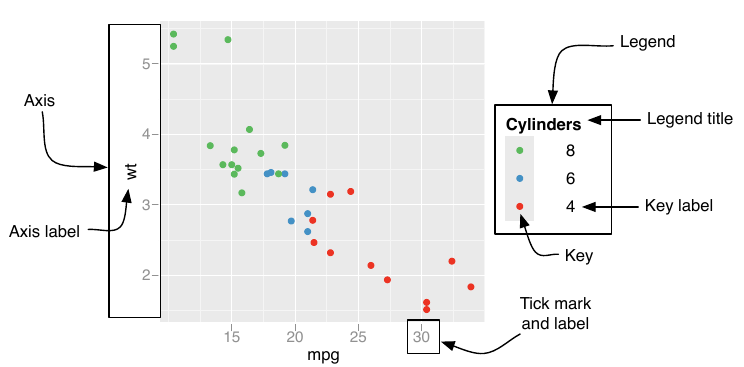
1.9.2 Legend merging and splitting

1.9.3 文本注释 text

Code
# 字体 样式
df <- data.frame(x = 1:3, y = 1:3, 
                 family = c("sans", "serif", "mono"),
                 face = c("plain", "bold", "italic"))
ggplot(df, aes(x, y)) + 
  geom_text(mapping = aes(label = paste0(family,": ",face), 
                          family = family, fontface = face),
            vjust = "inward", hjust = "inward")

Code

# 位置
df <- data.frame(
  x = c(1, 1, 2, 2, 1.5),
  y = c(1, 2, 1, 2, 1.5),
  text = c(
    "bottom-left", "top-left",  
    "bottom-right", "top-right", "center"
  )
)
ggplot(df, aes(x, y)) +
  geom_text(aes(label = text), vjust = "inward", hjust = "inward")

Code


# 自定义
df <- data.frame(
  treatment = c("a", "b", "c"), 
  response = c(1.2, 3.4, 2.5)
)
ggplot(df, aes(treatment, response)) + 
  geom_point() + 
  geom_text(
    mapping = aes(label = paste0("(", response, ")")), 
    nudge_x = -0.3,
    nudge_y=.2
  ) 

Code
label_info <- mpg |>
    group_by(drv) |>
    arrange(desc(displ)) |>
    slice_head(n = 1)|>
    mutate(
        drive_type = case_when(       # vectorise multiple if_else () statements 
        drv == "f" ~ "front-wheel drive",
        drv == "r" ~ "rear-wheel drive",
        drv == "4" ~ "4-wheel drive")
        )|>
    dplyr::select(displ, hwy, drv, drive_type)

p <-ggplot(mpg, aes(x = displ, y = hwy, color = drv)) +
    geom_point(alpha = 0.3) +
    geom_smooth(method="lm",formula="y~x",se = FALSE) +
    theme(legend.position = "none")

p+  geom_text(#添加注释  geom_label 标签加背景框
    data = label_info, 
    aes(x = displ, y = hwy, label = drive_type),#label映射
    fontface = "bold", size = 5, nudge_y = 2
    )

Code

p + ggrepel::geom_label_repel(                   
    data = label_info, 
    aes(x = displ, y = hwy, label = drive_type),
    fontface = "bold", size = 5, nudge_y = 2
  ) 

Code


potential_outliers <- mpg |>
  dplyr::filter(hwy > 40 | (hwy > 20 & displ > 5))

ggplot(mpg, aes(x = displ, y = hwy)) +
  geom_point() +
  ggrepel::geom_text_repel(data = potential_outliers, aes(label = model)) +
  geom_point(data = potential_outliers, color = "red") +
  geom_point(
    data = potential_outliers,
    color = "red", size = 3, shape = "circle open"
  )

1.9.4 参考线:线段 直线 箭头

geom_hline()

geom_vline()

geom_abline

geom_segment() arrow

Code
trend_text <- "Larger engine sizes tend to have lower fuel economy." |>
  str_wrap(width = 30)
trend_text
#> [1] "Larger engine sizes tend to\nhave lower fuel economy."
ggplot(mpg, aes(x = displ, y = hwy)) +
  geom_point() +
  annotate(
    geom = "label", x = 3.5, y = 38,
    label = trend_text,
    hjust = "left", color = "red"
  ) +
  annotate(
    geom = "segment",
    x = 3, y = 35, xend = 5, yend = 25, color = "red",
    arrow = arrow(type = "closed")
  )

Code
p <- ggplot(mpg, aes(displ, hwy)) +
  geom_point(
    data = dplyr::filter(mpg, manufacturer == "subaru"), 
    colour = "orange",
    size = 3
  ) +
  geom_point() 
p|p + 
  annotate(geom = "point", x = 5.5, y = 40, colour = "orange", size = 3) + 
  annotate(geom = "point", x = 5.5, y = 40) + 
  annotate(geom = "text", x = 5.6, y = 40, label = "subaru", hjust = "left")|
p + 
  annotate(
    geom = "curve", x = 4, y = 35, xend = 2.65, yend = 27, 
    curvature = .3, arrow = arrow(length = unit(2, "mm"))
  ) +
  annotate(geom = "text", x = 4.1, y = 35, label = "subaru", hjust = "left")

1.9.5 富文本/markdown

Code
df <- data.frame(x = 1:3, y = 1:3)
base <- ggplot(df, aes(x, y)) + 
  geom_point() + 
  labs(x = "Axis title with *italics* and **bold**")


library(ggtext)
base |
base + 
  geom_richtext(aes(x = 2, y = 3,
                    label =  "**title** of <span style = 'color:red'>xy</span>"),
                angle =-25)  + theme(axis.title.x = ggtext::element_markdown()) 
#> Warning in geom_richtext(aes(x = 2, y = 3, label = "**title** of <span style = 'color:red'>xy</span>"), : All aesthetics have length 1, but the data has 3 rows.
#> ℹ Please consider using `annotate()` or provide this layer with data containing
#>   a single row.

1.9.6 数学表达式

?plotmath

Code

tibble(
  x = 1:10,
  y = cumsum(x^2)) %>% 
  ggplot(aes(x, y)) +
  geom_point() +
  labs(
    x = quote(x[i]),
    y = quote(sum(x[i] ^ 2, i == 1, n)) #数学方程式
  )

Code

values <- seq(from = -2, to = 2, by = .01)
df <- tibble(x = values, y = values ^ 3)
ggplot(df, aes(x, y)) + 
  geom_path() + 
  labs(y = quote(f(x) == x^3))         #数学表达式   ?plotmath

1.10 Facet

Code
q <- ggplot(mpg,aes(x=displ))+
  geom_histogram(fill="lightblue")

# 一个分类变量
q + facet_wrap(~drv,nrow = 3)
#> `stat_bin()` using `bins = 30`. Pick better value `binwidth`.

Code
q + facet_wrap(~drv,ncol = 3)  #
#> `stat_bin()` using `bins = 30`. Pick better value `binwidth`.

Code

# 多个分类变量
q + facet_grid(drv~class)
#> `stat_bin()` using `bins = 30`. Pick better value `binwidth`.

Code
q + facet_grid(drv~.)
#> `stat_bin()` using `bins = 30`. Pick better value `binwidth`.

Code
q + facet_grid(.~drv)   #
#> `stat_bin()` using `bins = 30`. Pick better value `binwidth`.

Code
ggplot(mpg, aes(x = displ, y = hwy)) + 
  geom_point() + 
  facet_grid(drv ~ cyl) |
ggplot(mpg, aes(x = displ, y = hwy)) + 
  geom_point() + 
  facet_grid(drv ~ cyl, scales = "free_y")

1.11 Themes

plot, axis, legend, panel and facet

1.11.1 Plot elements + panel

Element Setter Description
plot.background element_rect() plot background
plot.title element_text() plot title
plot.margin margin() margins around plot
panel.background element_rect() panel background (under data)
panel.border element_rect() panel border (over data)
panel.grid.major element_line() major grid lines
panel.grid.major.x element_line() vertical major grid lines
panel.grid.major.y element_line() horizontal major grid lines
panel.grid.minor element_line() minor grid lines
panel.grid.minor.x element_line() vertical minor grid lines
panel.grid.minor.y element_line() horizontal minor grid lines
aspect.ratio numeric plot aspect ratio
Code
library(ggplot2)

base <- ggplot() +
  stat_function(fun = dnorm, geom = "density",
                xlim = c(-4, 4),
                fill = rgb(0, 0, 1, 0.1))


base + theme(
    plot.background = element_rect(
        colour = "red",
        fill = "lightblue",
        # 默认 fill = NA
        linewidth = 2,
    ),
    plot.margin = margin(
        t = 2,
        # Top margin
        r = 2,
        # Right margin
        b = 2,
        # Bottom margin
        l = 2
    )# Left margin
) +  theme(
    panel.background = element_rect(fill = "lightyellow"),
    panel.grid.major.y = element_line(color = "green", linewidth = 0.8),
    panel.grid.major.x = element_line(color = "purple", linewidth = 0.8))

1.11.2 Legend elements

Element Setter Description
legend.background element_rect() legend background
legend.key element_rect() background of legend keys
legend.key.size unit() legend key size
legend.key.height unit() legend key height
legend.key.width unit() legend key width
legend.margin unit() legend margin
legend.text element_text() legend labels
legend.text.align 0–1 legend label alignment (0 = right, 1 = left)
legend.title element_text() legend name
legend.title.align 0–1 legend name alignment (0 = right, 1 = left)
Code
df <- data.frame(x = 1:4, y = 1:4, z = rep(c("a", "b"), each = 2))
base <- ggplot(df, aes(x, y, colour = z)) + geom_point()

base + theme(
  legend.background = element_rect(
    fill = "lemonchiffon", 
    colour = "grey50", 
    linewidth = 1
  )
)

Code
base + theme(
  legend.key = element_rect(color = "grey50"),
  legend.key.width = unit(0.9, "cm"),
  legend.key.height = unit(0.75, "cm")
)

Code
base + theme(
  legend.text = element_text(size = 15),
  legend.title = element_text(size = 15, face = "bold")
)

Code

base + 
  theme(legend.position = "top") +
  guides(color = guide_legend(nrow = 3))

Code
base + 
  theme(legend.position = "bottom") +
  guides(color = guide_legend(nrow = 2, override.aes = list(size = 4)))

Code

# 文本

ggplot(mtcars, aes(wt, mpg, color = factor(cyl))) +
  geom_point(size=3) +
  scale_color_discrete(name="Cylinders") +
  theme(legend.position = c(.95, .95),
        legend.justification = c(1, 1),
        legend.background = element_rect(fill = "lightgrey",
                                         color = "white",
                                         linewidth = 1),
        legend.key = element_blank(),
        legend.direction = "horizontal")

1.11.3 Axis elements

Element Setter Description
axis.line element_line() line parallel to axis (hidden in default themes)
axis.text element_text() tick labels
axis.text.x element_text() x-axis tick labels
axis.text.y element_text() y-axis tick labels
axis.title element_text() axis titles
axis.title.x element_text() x-axis title
axis.title.y element_text() y-axis title
axis.ticks element_line() axis tick marks
axis.ticks.length unit() length of tick marks

1.12 字体

Code
findfont <- function(x){
  suppressMessages(require(showtext))
  suppressMessages(require(dplyr))
  dplyr::filter(font_files(), grepl(x, family, ignore.case=TRUE)) |> 
    dplyr::select(path, file, family, face)
}

findfont("comic")
#>               path        file        family        face
#> 1 C:/Windows/Fonts   comic.ttf Comic Sans MS     Regular
#> 2 C:/Windows/Fonts comicbd.ttf Comic Sans MS        Bold
#> 3 C:/Windows/Fonts  comici.ttf Comic Sans MS      Italic
#> 4 C:/Windows/Fonts  comicz.ttf Comic Sans MS Bold Italic
font_add(family = "Times New Roman", regular = "C:\\Windows\\Fonts\\Times New Roman\\times.ttf",
         bold = "C:\\Windows\\Fonts\\Times New Roman\\timesbd.ttf",
         italic = "C:\\Windows\\Fonts\\Times New Roman\\timesi.ttf",
         bolditalic = "C:\\Windows\\Fonts\\Times New Roman\\timesbi.ttf")
findfont("Times New Roman")
#>               path        file          family        face
#> 1 C:/Windows/Fonts   times.ttf Times New Roman     Regular
#> 2 C:/Windows/Fonts timesbd.ttf Times New Roman        Bold
#> 3 C:/Windows/Fonts timesbi.ttf Times New Roman Bold Italic
#> 4 C:/Windows/Fonts  timesi.ttf Times New Roman      Italic
font_families()
#> [1] "sans"            "serif"           "mono"            "wqy-microhei"   
#> [5] "Times New Roman"
Code
ggplot(mpg, aes(x = displ, y = hwy, color = drv)) +
  geom_point() +
  labs(
    title = "Larger engine sizes tend to have lower fuel economy",
    caption = "Source: https://fueleconomy.gov."
  ) +
  theme(
    legend.position = c(0.8, 0.9),
    legend.direction = "horizontal",
    legend.box.background = element_rect(color = "blue"),
    plot.title = element_text(face = "bold",hjust = 0.5),
    plot.title.position = "plot",
    plot.caption.position = "plot",
    plot.caption = element_text(hjust = 1)
  )

Back to top