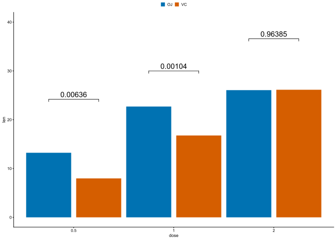
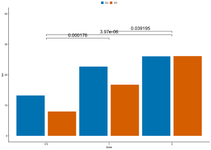
显著性——差异比较
Code
library(ggplot2)
pal <- c("#0072B2", "#D55E00","#122cad")

theme_nature <- theme_classic(base_size = 6.5, base_family = "sans") +
  theme(
    axis.line        = element_line(linewidth = 0.35, colour = "black"),
    axis.ticks       = element_line(linewidth = 0.35, colour = "black"),
    axis.title       = element_text(size = 6.5),
    axis.text        = element_text(size = 6.0),
    legend.title     = element_blank(),
    legend.text      = element_text(size = 6.0),
    legend.position  = "top",
    legend.direction = "horizontal",
    legend.justification = "center",
    legend.margin    = margin(0, 0, 2, 0, "pt"),
    legend.key.size  = unit(2.4, "mm"),
    panel.grid       = element_blank()
  )


df <- ToothGrowth

df
#>     len supp dose
#> 1   4.2   VC  0.5
#> 2  11.5   VC  0.5
#> 3   7.3   VC  0.5
#> 4   5.8   VC  0.5
#> 5   6.4   VC  0.5
#> 6  10.0   VC  0.5
#> 7  11.2   VC  0.5
#> 8  11.2   VC  0.5
#> 9   5.2   VC  0.5
#> 10  7.0   VC  0.5
#> 11 16.5   VC  1.0
#> 12 16.5   VC  1.0
#> 13 15.2   VC  1.0
#> 14 17.3   VC  1.0
#> 15 22.5   VC  1.0
#> 16 17.3   VC  1.0
#> 17 13.6   VC  1.0
#> 18 14.5   VC  1.0
#> 19 18.8   VC  1.0
#> 20 15.5   VC  1.0
#> 21 23.6   VC  2.0
#> 22 18.5   VC  2.0
#> 23 33.9   VC  2.0
#> 24 25.5   VC  2.0
#> 25 26.4   VC  2.0
#> 26 32.5   VC  2.0
#> 27 26.7   VC  2.0
#> 28 21.5   VC  2.0
#> 29 23.3   VC  2.0
#> 30 29.5   VC  2.0
#> 31 15.2   OJ  0.5
#> 32 21.5   OJ  0.5
#> 33 17.6   OJ  0.5
#> 34  9.7   OJ  0.5
#> 35 14.5   OJ  0.5
#> 36 10.0   OJ  0.5
#> 37  8.2   OJ  0.5
#> 38  9.4   OJ  0.5
#> 39 16.5   OJ  0.5
#> 40  9.7   OJ  0.5
#> 41 19.7   OJ  1.0
#> 42 23.3   OJ  1.0
#> 43 23.6   OJ  1.0
#> 44 26.4   OJ  1.0
#> 45 20.0   OJ  1.0
#> 46 25.2   OJ  1.0
#> 47 25.8   OJ  1.0
#> 48 21.2   OJ  1.0
#> 49 14.5   OJ  1.0
#> 50 27.3   OJ  1.0
#> 51 25.5   OJ  2.0
#> 52 26.4   OJ  2.0
#> 53 22.4   OJ  2.0
#> 54 24.5   OJ  2.0
#> 55 24.8   OJ  2.0
#> 56 30.9   OJ  2.0
#> 57 26.4   OJ  2.0
#> 58 27.3   OJ  2.0
#> 59 29.4   OJ  2.0
#> 60 23.0   OJ  2.0
str(df)
#> 'data.frame':    60 obs. of  3 variables:
#>  $ len : num  4.2 11.5 7.3 5.8 6.4 10 11.2 11.2 5.2 7 ...
#>  $ supp: Factor w/ 2 levels "OJ","VC": 2 2 2 2 2 2 2 2 2 2 ...
#>  $ dose: num  0.5 0.5 0.5 0.5 0.5 0.5 0.5 0.5 0.5 0.5 ...

df$dose <- as.character(df$dose)
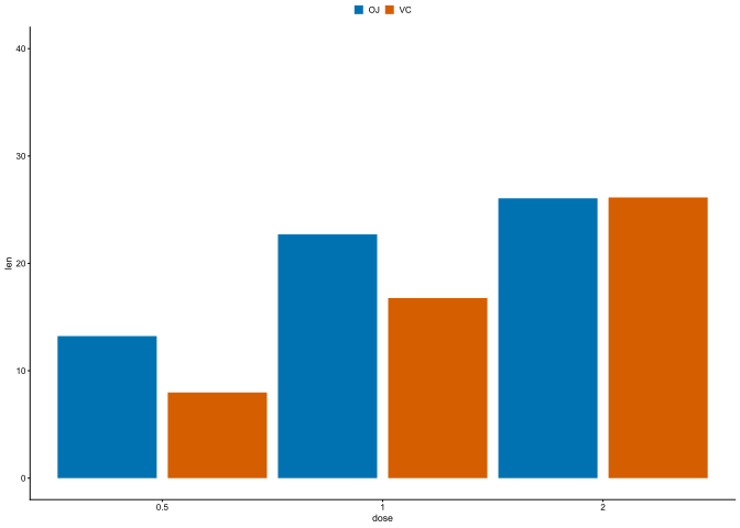
p <- ggplot(data = df,mapping = aes(dose,len,fill = supp)) +
  geom_bar(stat = "summary", fun = "mean",position = position_dodge(1))+
  coord_cartesian(ylim = c(0, 40))+
  scale_fill_manual(values = pal) +
  theme_nature
p
Code
https://r-graphics.org/RECIPE-ANNOTATE-SEGMENT.html
Code
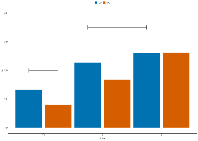
p + annotate("segment", x = 0.75, xend = 1.25, y = 20, yend = 20,
           arrow = arrow(ends = "both", angle = 90, length = unit(.2,"cm")))+
    annotate("segment", x = 1.75, xend = 2.75, y = 35, yend = 35,
           arrow = arrow(ends = "both", angle = 90, length = unit(.2,"cm")))
Code
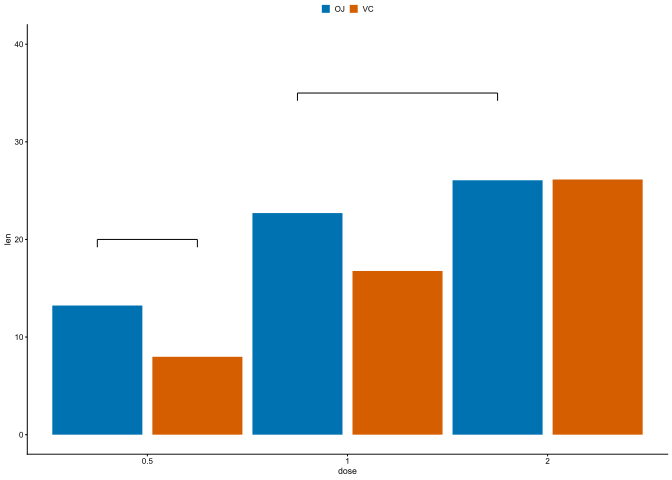
p +
  # 括号1:剂量 0.5 组,OJ(0.75) ↔ VC(1.25),y = 20
  annotate("segment", x = 0.75, xend = 1.25, y = 20, yend = 20, linewidth = 0.35) +
  annotate("segment", x = 0.75, xend = 0.75, y = 19.2, yend = 20, linewidth = 0.35) +
  annotate("segment", x = 1.25, xend = 1.25, y = 19.2, yend = 20, linewidth = 0.35) +
  # 括号2:x = 1.75 ↔ 2.75,y = 35
  annotate("segment", x = 1.75, xend = 2.75, y = 35, yend = 35, linewidth = 0.35) +
  annotate("segment", x = 1.75, xend = 1.75, y = 34.2, yend = 35, linewidth = 0.35) +
  annotate("segment", x = 2.75, xend = 2.75, y = 34.2, yend = 35, linewidth = 0.35)
Code
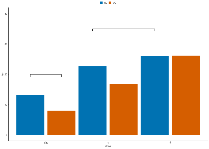
# 括号数据框:每条括号 3 段 = 1 条横线 + 2 条向下竖线
brackets <- data.frame(
  x    = c(0.75, 0.75, 1.25, 1.75, 1.75, 2.75),   # 每段起点 x
  xend = c(1.25, 0.75, 1.25, 2.75, 1.75, 2.75),   # 每段终点 x
  y    = c(20,   20,   20,   35,   35,   35),      # 每段起点 y
  yend = c(20,   19.2, 19.2, 35,   34.2, 34.2)     # 每段终点 y(竖线向下)
)

p + geom_segment(data = brackets,
                 aes(x = x, y = y, xend = xend, yend = yend),
                 linewidth = 0.35, inherit.aes = FALSE)
l
Back to top