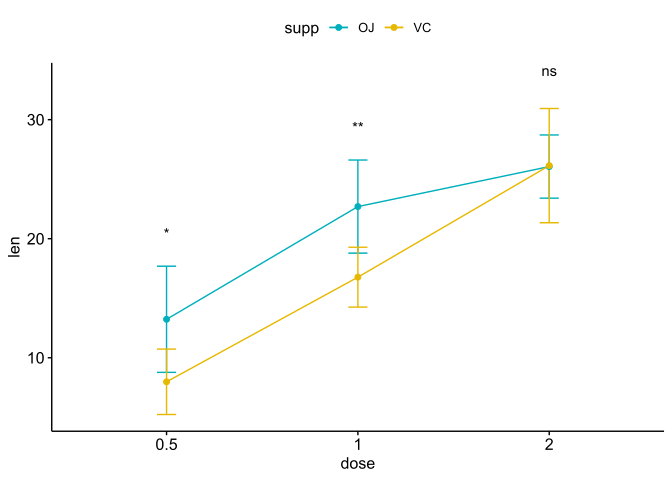
1 折线图
Code
f4h <-read_excel("data/01source.xlsx", sheet = "Fig.4", range = "A20:P23")
colnames(f4h) <-
    c("Days", rep(
        c("PBS", "SLAMF6+ PD-1+ CD8+ cells", "SLAMF6- PD-1+ CD8+ cells"),
        each = 5
    ))

f4h |> pivot_longer(cols = -1,
                    names_to = "method",
                    values_to = "volume",) |>
    dplyr::mutate(id=factor(rep(1:15,3)),
                  Days = factor(Days, levels = c("-1", "7", "14")),
                  method = factor(
                      method,
                      levels = c("PBS", "SLAMF6+ PD-1+ CD8+ cells",
                                 "SLAMF6- PD-1+ CD8+ cells")
                  )) -> f4h
f4h
#> # A tibble: 45 × 4
#>    Days  method                   volume id
#>    <fct> <fct>                     <dbl> <fct>
#>  1 -1    PBS                        19.2 1
#>  2 -1    PBS                        27.0 2
#>  3 -1    PBS                        23.4 3
#>  4 -1    PBS                        27.9 4
#>  5 -1    PBS                        29.7 5
#>  6 -1    SLAMF6+ PD-1+ CD8+ cells   31.9 6
#>  7 -1    SLAMF6+ PD-1+ CD8+ cells   34.5 7
#>  8 -1    SLAMF6+ PD-1+ CD8+ cells   44.4 8
#>  9 -1    SLAMF6+ PD-1+ CD8+ cells   29.1 9
#> 10 -1    SLAMF6+ PD-1+ CD8+ cells   41.4 10
#> # ℹ 35 more rows
统计p值
Code
# 重复测量方差设计
library(nlme)
model <- lme(volume ~ method*Days, random = ~1|id/Days, data = f4h)
summary(model)
#> Linear mixed-effects model fit by REML
#>   Data: f4h
#>        AIC      BIC    logLik
#>   304.5845 323.5868 -140.2923
#>
#> Random effects:
#>  Formula: ~1 | id
#>         (Intercept)
#> StdDev:    4.346709
#>
#>  Formula: ~1 | Days %in% id
#>         (Intercept) Residual
#> StdDev:    8.366812 3.060766
#>
#> Fixed effects:  volume ~ method * Days
#>                                           Value Std.Error DF   t-value p-value
#> (Intercept)                            25.43718  4.433186 24  5.737900  0.0000
#> methodSLAMF6+ PD-1+ CD8+ cells         10.81993  6.269472 12  1.725813  0.1100
#> methodSLAMF6- PD-1+ CD8+ cells          4.63341  6.269472 12  0.739043  0.4741
#> Days7                                   9.55505  5.634601 24  1.695781  0.1029
#> Days14                                 22.41864  5.634601 24  3.978745  0.0006
#> methodSLAMF6+ PD-1+ CD8+ cells:Days7  -37.58056  7.968529 24 -4.716123  0.0001
#> methodSLAMF6- PD-1+ CD8+ cells:Days7   -8.90525  7.968529 24 -1.117552  0.2748
#> methodSLAMF6+ PD-1+ CD8+ cells:Days14 -55.79891  7.968529 24 -7.002410  0.0000
#> methodSLAMF6- PD-1+ CD8+ cells:Days14 -14.68420  7.968529 24 -1.842774  0.0777
#>  Correlation:
#>                                       (Intr) mtSLAMF6+PD-1+CD8+c
#> methodSLAMF6+ PD-1+ CD8+ cells        -0.707
#> methodSLAMF6- PD-1+ CD8+ cells        -0.707  0.500
#> Days7                                 -0.636  0.449
#> Days14                                -0.636  0.449
#> methodSLAMF6+ PD-1+ CD8+ cells:Days7   0.449 -0.636
#> methodSLAMF6- PD-1+ CD8+ cells:Days7   0.449 -0.318
#> methodSLAMF6+ PD-1+ CD8+ cells:Days14  0.449 -0.636
#> methodSLAMF6- PD-1+ CD8+ cells:Days14  0.449 -0.318
#>                                       mtSLAMF6-PD-1+CD8+c Days7  Days14
#> methodSLAMF6+ PD-1+ CD8+ cells
#> methodSLAMF6- PD-1+ CD8+ cells
#> Days7                                  0.449
#> Days14                                 0.449               0.500
#> methodSLAMF6+ PD-1+ CD8+ cells:Days7  -0.318              -0.707 -0.354
#> methodSLAMF6- PD-1+ CD8+ cells:Days7  -0.636              -0.707 -0.354
#> methodSLAMF6+ PD-1+ CD8+ cells:Days14 -0.318              -0.354 -0.707
#> methodSLAMF6- PD-1+ CD8+ cells:Days14 -0.636              -0.354 -0.707
#>                                       mSLAMF6+PD-1+CD8+c:D7
#> methodSLAMF6+ PD-1+ CD8+ cells
#> methodSLAMF6- PD-1+ CD8+ cells
#> Days7
#> Days14
#> methodSLAMF6+ PD-1+ CD8+ cells:Days7
#> methodSLAMF6- PD-1+ CD8+ cells:Days7   0.500
#> methodSLAMF6+ PD-1+ CD8+ cells:Days14  0.500
#> methodSLAMF6- PD-1+ CD8+ cells:Days14  0.250
#>                                       mSLAMF6-PD-1+CD8+c:D7
#> methodSLAMF6+ PD-1+ CD8+ cells
#> methodSLAMF6- PD-1+ CD8+ cells
#> Days7
#> Days14
#> methodSLAMF6+ PD-1+ CD8+ cells:Days7
#> methodSLAMF6- PD-1+ CD8+ cells:Days7
#> methodSLAMF6+ PD-1+ CD8+ cells:Days14  0.250
#> methodSLAMF6- PD-1+ CD8+ cells:Days14  0.500
#>                                       mSLAMF6+PD-1+CD8+c:D1
#> methodSLAMF6+ PD-1+ CD8+ cells
#> methodSLAMF6- PD-1+ CD8+ cells
#> Days7
#> Days14
#> methodSLAMF6+ PD-1+ CD8+ cells:Days7
#> methodSLAMF6- PD-1+ CD8+ cells:Days7
#> methodSLAMF6+ PD-1+ CD8+ cells:Days14
#> methodSLAMF6- PD-1+ CD8+ cells:Days14  0.500
#>
#> Standardized Within-Group Residuals:
#>         Min          Q1         Med          Q3         Max
#> -0.62401382 -0.15515176 -0.03440848  0.17260010  0.72287328
#>
#> Number of Observations: 45
#> Number of Groups:
#>           id Days %in% id
#>           15           45
df_aov <- anova(model)
df_aov
#>             numDF denDF   F-value p-value
#> (Intercept)     1    24 263.95442  <.0001
#> method          2    12  13.12729  0.0010
#> Days            2    24   1.89320  0.1724
#> method:Days     4    24  13.74242  <.0001

#成对比较
library(emmeans)
method_means <- emmeans(model, ~method)
print(method_means)
#>  method                   emmean   SE df lower.CL upper.CL
#>  PBS                        36.1 3.01 14    29.64     42.6
#>  SLAMF6+ PD-1+ CD8+ cells   15.8 3.01 12     9.23     22.4
#>  SLAMF6- PD-1+ CD8+ cells   32.9 3.01 12    26.30     39.4
#>
#> Results are averaged over the levels of: Days
#> Degrees-of-freedom method: containment
#> Confidence level used: 0.95
method_comparisons <- pairs(method_means)
method_comparisons
#>  contrast                                                estimate   SE df
#>  PBS - (SLAMF6+ PD-1+ CD8+ cells)                           20.31 4.26 12
#>  PBS - (SLAMF6- PD-1+ CD8+ cells)                            3.23 4.26 12
#>  (SLAMF6+ PD-1+ CD8+ cells) - (SLAMF6- PD-1+ CD8+ cells)   -17.08 4.26 12
#>  t.ratio p.value
#>    4.768  0.0012
#>    0.758  0.7345
#>   -4.009  0.0046
#>
#> Results are averaged over the levels of: Days
#> Degrees-of-freedom method: containment
#> P value adjustment: tukey method for comparing a family of 3 estimates
2 ggplot2
Code
pvalue <- method_comparisons |> broom::tidy() |>
    dplyr::select(contrast, adj.p.value) |>
    dplyr::mutate(padj=round(adj.p.value,digits = 4),
                  p_adj_sci=format(adj.p.value,scientific = T,digits = 4))

pvalue
#> # A tibble: 3 × 4
#>   contrast                                          adj.p.value   padj p_adj_sci
#>   <chr>                                                   <dbl>  <dbl> <chr>
#> 1 PBS - (SLAMF6+ PD-1+ CD8+ cells)                      0.00123 0.0012 1.230e-03
#> 2 PBS - (SLAMF6- PD-1+ CD8+ cells)                      0.735   0.734  7.345e-01
#> 3 (SLAMF6+ PD-1+ CD8+ cells) - (SLAMF6- PD-1+ CD8+…     0.00456 0.0046 4.558e-03

p <- f4h |> summarise(
    mean_volume = mean(volume),
    sd = sd(volume),
    .by = c(Days, method),) |>
    ggplot(aes(
        x = Days,
        y = mean_volume,
        color = method,
        group = method,)) +
    geom_errorbar(
        aes(ymin = mean_volume - sd, ymax = mean_volume + sd),
        position = position_dodge(0),
        width = .2,
        linewidth = 0.5,
    ) +
    geom_line(position = position_dodge(0),
              linewidth = 0.8) +
    geom_point(
        aes(shape = method),
        position = position_dodge(0),
        color = "black",
        size = 2) +
    theme_pubr() +
    theme(legend.title = element_blank())

# 使用ggplot_build()获取图层数据
plot_data <- ggplot_build(p)

# 查看X轴的数值坐标
plot_data$data
#> [[1]]
#>         ymin      ymax x         y  colour group PANEL flipped_aes      xmin
#> 1 21.2341315 29.640231 1 25.437181 #F8766D     1     1       FALSE 0.9666667
#> 2 29.8251093 42.689121 1 36.257115 #00BA38     2     1       FALSE 0.9666667
#> 3 23.2386460 36.902540 1 30.070593 #619CFF     3     1       FALSE 0.9666667
#> 4 20.3358912 49.648564 2 34.992228 #F8766D     1     1       FALSE 1.9666667
#> 5  4.8856152 11.577581 2  8.231598 #00BA38     2     1       FALSE 1.9666667
#> 6 22.3836755 39.057109 2 30.720392 #619CFF     3     1       FALSE 1.9666667
#> 7 28.7160676 66.995581 3 47.855824 #F8766D     1     1       FALSE 2.9666667
#> 8  0.5880804  5.165626 3  2.876853 #00BA38     2     1       FALSE 2.9666667
#> 9 27.2406302 48.369439 3 37.805035 #619CFF     3     1       FALSE 2.9666667
#>       xmax order linewidth linetype width alpha
#> 1 1.033333     1       0.5        1   0.2    NA
#> 2 1.033333     2       0.5        1   0.2    NA
#> 3 1.033333     3       0.5        1   0.2    NA
#> 4 2.033333     1       0.5        1   0.2    NA
#> 5 2.033333     2       0.5        1   0.2    NA
#> 6 2.033333     3       0.5        1   0.2    NA
#> 7 3.033333     1       0.5        1   0.2    NA
#> 8 3.033333     2       0.5        1   0.2    NA
#> 9 3.033333     3       0.5        1   0.2    NA
#>
#> [[2]]
#>   x         y  colour group PANEL flipped_aes order xmin xmax      ymax
#> 1 1 25.437181 #F8766D     1     1       FALSE     1    1    1 25.437181
#> 2 2 34.992228 #F8766D     1     1       FALSE     1    2    2 34.992228
#> 3 3 47.855824 #F8766D     1     1       FALSE     1    3    3 47.855824
#> 4 1 36.257115 #00BA38     2     1       FALSE     2    1    1 36.257115
#> 5 2  8.231598 #00BA38     2     1       FALSE     2    2    2  8.231598
#> 6 3  2.876853 #00BA38     2     1       FALSE     2    3    3  2.876853
#> 7 1 30.070593 #619CFF     3     1       FALSE     3    1    1 30.070593
#> 8 2 30.720392 #619CFF     3     1       FALSE     3    2    2 30.720392
#> 9 3 37.805035 #619CFF     3     1       FALSE     3    3    3 37.805035
#>   linewidth linetype alpha
#> 1       0.8        1    NA
#> 2       0.8        1    NA
#> 3       0.8        1    NA
#> 4       0.8        1    NA
#> 5       0.8        1    NA
#> 6       0.8        1    NA
#> 7       0.8        1    NA
#> 8       0.8        1    NA
#> 9       0.8        1    NA
#>
#> [[3]]
#>   shape x         y group PANEL order xmin xmax      ymax colour fill size
#> 1    16 1 25.437181     1     1     1    1    1 25.437181  black   NA    2
#> 2    17 1 36.257115     2     1     2    1    1 36.257115  black   NA    2
#> 3    15 1 30.070593     3     1     3    1    1 30.070593  black   NA    2
#> 4    16 2 34.992228     1     1     1    2    2 34.992228  black   NA    2
#> 5    17 2  8.231598     2     1     2    2    2  8.231598  black   NA    2
#> 6    15 2 30.720392     3     1     3    2    2 30.720392  black   NA    2
#> 7    16 3 47.855824     1     1     1    3    3 47.855824  black   NA    2
#> 8    17 3  2.876853     2     1     2    3    3  2.876853  black   NA    2
#> 9    15 3 37.805035     3     1     3    3    3 37.805035  black   NA    2
#>   alpha    stroke
#> 1    NA 0.5454545
#> 2    NA 0.5454545
#> 3    NA 0.5454545
#> 4    NA 0.5454545
#> 5    NA 0.5454545
#> 6    NA 0.5454545
#> 7    NA 0.5454545
#> 8    NA 0.5454545
#> 9    NA 0.5454545


p  +  annotate(geom = "segment",
               x = 3.4,
               y = 47.855824,
               yend = 2.876853,) + annotate(
                   geom = "text",
                   x = 3.45,
                   y = (47.855824 + 2.876853) / 2,
                   angle = 270,
                   label = pvalue$padj[1],
               ) +
    annotate(geom = "segment",
             x = 3.15,
             y = 47.855824,
             yend = 37.805035,) + annotate(
                 geom = "text",
                 x = 3.2,
                 y = (47.855824 + 37.805035) / 2,
                 angle = 270,
                 label = pvalue$padj[2],
             ) +
    annotate(geom = "segment",
             x = 3.3,
             y = 2.876853,
             yend = 37.805035,) + annotate(
                 geom = "text",
                 x = 3.35,
                 y = (2.876853 + 37.805035) / 2,
                 angle = 270,
                 label = pvalue$padj[3],
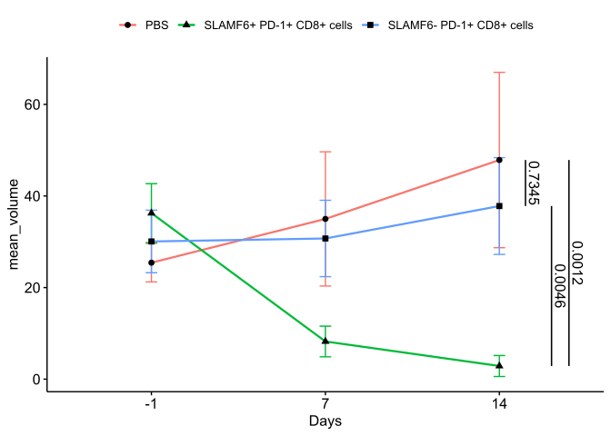
             )
Code
#y=c(47.855824,37.805035,2.876853,),
#yend = c(2.876853,47.855824,37.805035,),3 ggpubr
Code
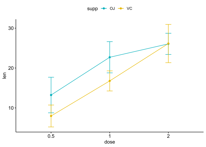
Code
# Add p-values onto the line plots
# Remove brackets using linetype = "blank"
stat.test <- stat.test %>%
    add_xy_position(fun = "mean_sd", x = "dose")
lp + stat_pvalue_manual(stat.test,
                        label = "p.adj.signif",
                        tip.length = 0,
                        linetype  = "blank")