Code
library(tidyverse)
p <- ggplot(data = mpg, aes(x=displ, y=hwy)) +
    geom_point()
p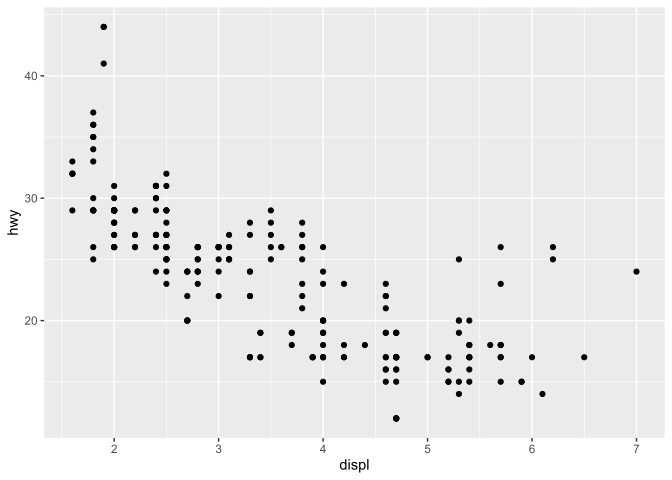
library(tidyverse)
p <- ggplot(data = mpg, aes(x=displ, y=hwy)) +
geom_point()
p
geom_dotplot()
ToothGrowth$dose <- as.factor(ToothGrowth$dose)
p1 <- ggplot(ToothGrowth, aes(x=dose, y=len)) +
  geom_dotplot(binaxis='y', binwidth = 0.4,stackdir='center',
               stackratio=1.5, dotsize=1.2)


p2<- p1 + stat_summary(fun=median, geom="point", shape=18,
                 size=3, color="red")

library(patchwork)
p1+p2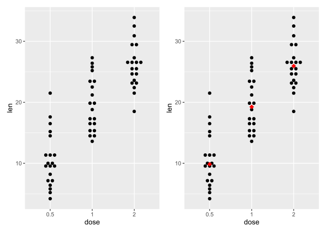
ggpubr::ggdotplot()
library(ggpubr)
library(readxl)
f6d <-
    read_excel("data/01source.xlsx", sheet = "Fig.6", range = "D2:E18")
f6d |> pivot_longer(
    cols = everything(),
    names_to = "status",
    values_to = "Ratio",
) |>
tidyr::drop_na() ->f6dggdotplot(f6d,
x="status",
y="Ratio",
add =c("mean_sd"),
color = "status",
fill = "status",
error.plot = "errorbar",
binwidth = 0.2
)+
geom_signif(
comparisons = list(c("relapse","non-relapse")),
)+
stat_summary(
fun.data = "mean_sd",geom = "pointrange",linewidth=.3
)+
ggplot2::annotate(
geom="segment",
x=0.9,
xend=1.1,
y=2.42019873,#均值
)+
ggplot2::annotate(
geom="segment",
x=1.9,
xend=2.1,
y=0.789463173,#均值
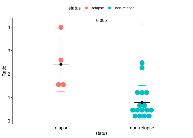
)
Beeswarm plots