https://bookdown.org/ks6017/GLM_bookdown3/
https://bookdown.org/roback/bookdown-BeyondMLR/
高级医学统计学 第15章 广义线性模型
在统计学上,广义线性模型 (generalized linear model, GLM)是一种应用灵活的线性回归模型。该模型允许因变量的误差分布有除了正态分布之外的其它分布。此模型假设实验者所测量的随机变量的分布函数与实验中系统性效应(即非随机的效应)可经由一链接函数(link function)建立可解释其相关性的函数。
在广义线性模式中,假设每个资料的观测值 Y 来自某个指数族分布 f 。
GLM 组件
广义线性模型是对线性模型的扩展,适用于非正态分布的数据,假设观测值之间是独立的,不能处理组内相关性。模型形式为:
\[
g(E(Y))=\mathbf{X} \beta
\]
线性预测器(Linear Predictor):
\[
\eta = \mathbf{X} \beta
\]
因变量的期望值与线性预测函数的关系:
\[
E(y)=\mu
\]
链接函数 g(.) :
\[
\eta =g(\mu)=g(E(y))
\]
反链接函数g-1 (.):
\[
E(y)=g^{-1}(\eta)
\]
y 的方差:
\[
Var(y)=f(\mu)=f(g^{-1}(\mathbf{X}\beta))
\]
典型链接函数
数据来源
数据下载网站
Show the code library ( tidyverse ) library ( patchwork ) df <- read_csv ( "data/Default.csv" ) df <- df %>% mutate ( across ( 1 : 2 , ~ factor ( .x ,levels = c ( "No" ,"Yes" ) ,labels = c ( 0 ,1 ) )
)
)
str ( df ) #> tibble [10,000 × 4] (S3: tbl_df/tbl/data.frame) #> $ default: Factor w/ 2 levels "0","1": 1 1 1 1 1 1 1 1 1 1 ... #> $ student: Factor w/ 2 levels "0","1": 1 2 1 1 1 2 1 2 1 1 ... #> $ balance: num [1:10000] 730 817 1074 529 786 ... #> $ income : num [1:10000] 44362 12106 31767 35704 38463 ... # 是否违约 是否学生 余额 收入 head ( df ) #> # A tibble: 6 × 4 #> default student balance income #> <fct> <fct> <dbl> <dbl> #> 1 0 0 730. 44362. #> 2 0 1 817. 12106. #> 3 0 0 1074. 31767. #> 4 0 0 529. 35704. #> 5 0 0 786. 38463. #> 6 0 1 920. 7492. table ( df $ default ,df $ student ) #> #> 0 1 #> 0 6850 2817 #> 1 206 127
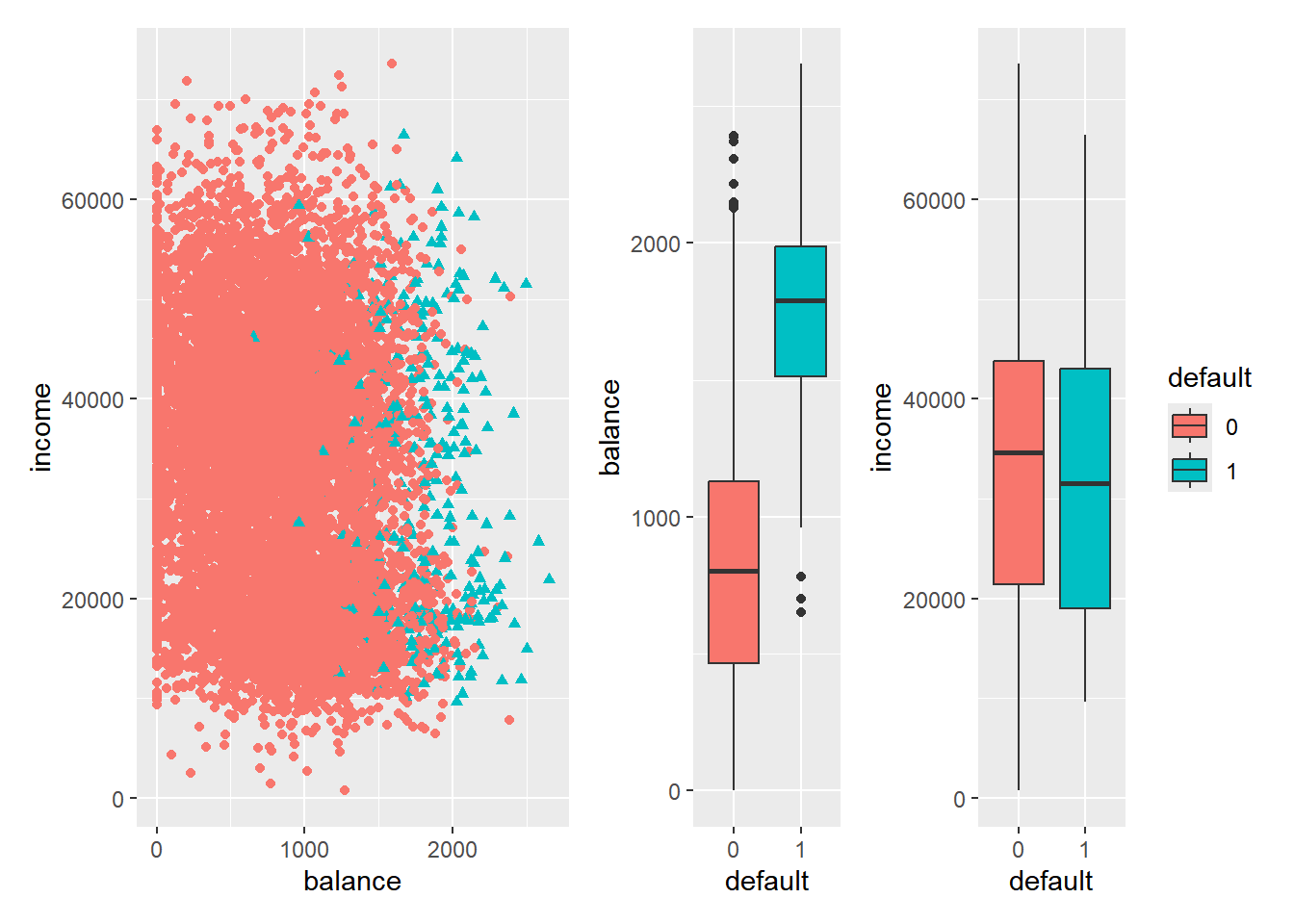
Show the code ggplot ( df ,aes ( balance ,income ) ) + geom_point ( aes ( shape= default ,color= default ) ,show.legend = F ) |
ggplot ( df ,aes ( default ,balance ,fill= default ) ,) + geom_boxplot ( show.legend = F ) +
ggplot ( df ,aes ( default ,income ,fill= default ) ) + geom_boxplot ( )
恒等链接线性回归
线性回归是一种简单的线性回归模型,其中假设响应变量服从正态分布,并且使用恒等链接函数(identity link function),t-statistic
Show the code library ( tidymodels ) library ( ggfortify ) # 使用 glm() 函数进行高斯线性回归 glm_gauss <- linear_reg ( ) %>% set_engine ( "glm" , family = stats :: gaussian ( link = "identity" ) ) %>%
fit ( as.numeric ( default ) - 1 ~ balance ,data= df )
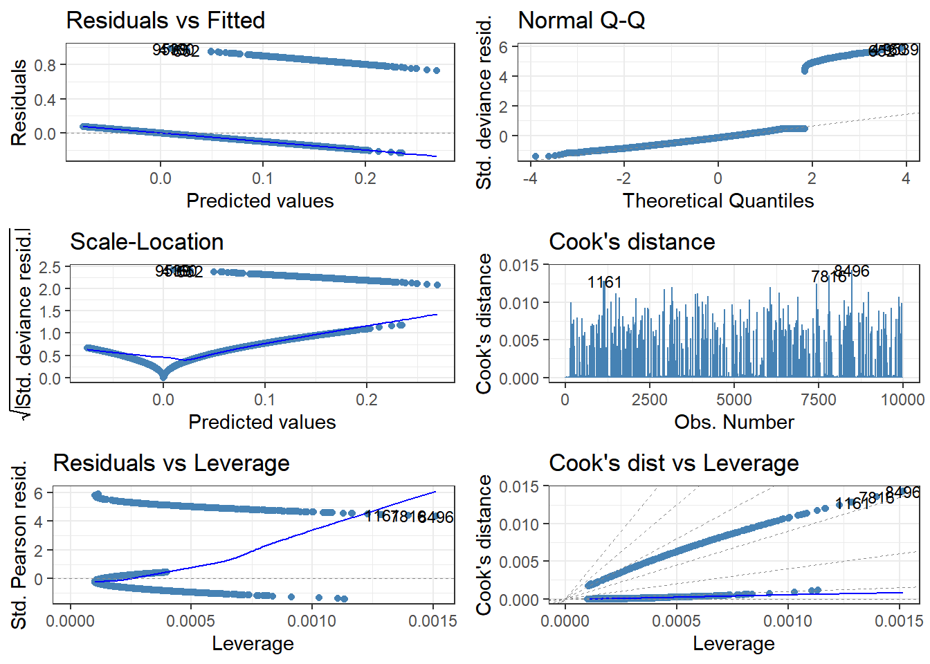
# 查看模型的系数 tidy ( glm_gauss ) #> # A tibble: 2 × 5 #> term estimate std.error statistic p.value #> <chr> <dbl> <dbl> <dbl> <dbl> #> 1 (Intercept) -0.0752 0.00335 -22.4 1.26e-108 #> 2 balance 0.000130 0.00000347 37.4 2.77e-286 # 查看模型性能的 AIC 和 Deviance glance ( glm_gauss ) %>% dplyr :: select ( AIC , deviance ) #> # A tibble: 1 × 2 #> AIC deviance #> <dbl> <dbl> #> 1 -7284. 282. # Change the theme and colour autoplot ( glm_gauss , which = 1 : 6 , ncol = 2 , label.size = 3 , colour = "steelblue" ) + theme_bw ( )
逻辑回归
逻辑回归用于处理分类问题。其模型假设响应变量的对数优势(log odds)服从线性模型。
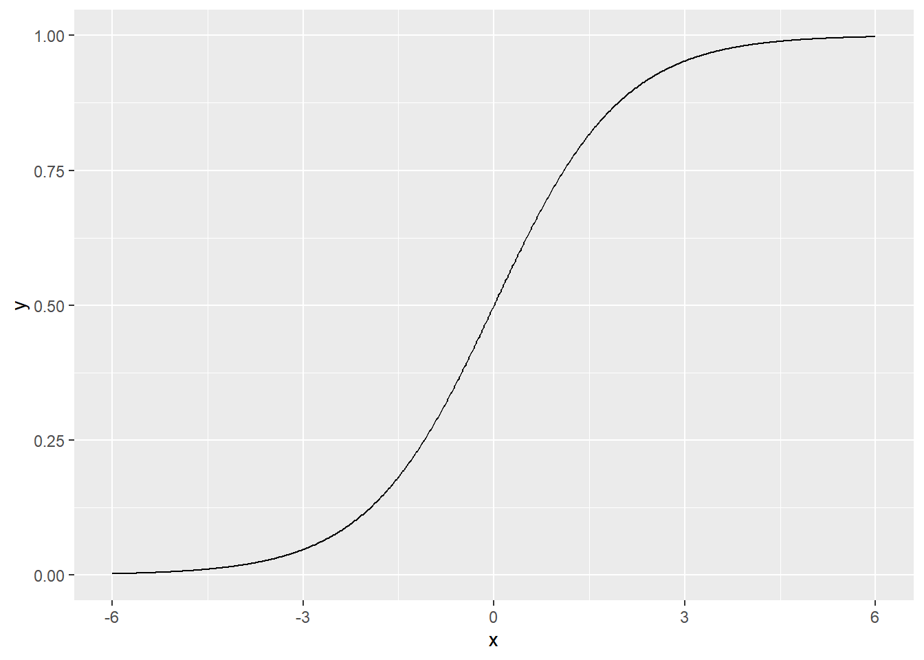
Sigmoid 激活函数:
\[
f(x)=\frac{1}{1+e^{-x}}=\frac{e^x}{1+e^x}
\]
逻辑回归( logistic regression )的一般表达式:
\[
\pi(Y=k|X=(X_1,X_2,...,X_p)=\frac{e^{\beta_{k0}+\beta_{k1}X_1+\beta_{k2}X_2+...+\beta_{kp}X_p}}{1+\sum_{l=1}^{K-1} e^{\beta_{l0}+\beta_{l1}X_1+\beta_{l2}X_2+...+\beta_{lp}X_p}}
\] 其中\(\pi\) 是成功概率,\(k=1,2,...,K-1\) 是因变量的第k个水平,共K 个水平,\(p\) 是自变量个数。
logit link function
z-statistic
二分类Binary
当\(K=2\) 时,\(k=l=p=1\) 即二分类逻辑回归,一般需要引入虚拟变量(哑变量,dummy variable),通常取值为 0或1。
极大似然法(maximum likelihood),likelihood function :
\[
\ell (\beta_0,\beta_1)=\prod_{i:y_i=1}\pi(x_i)\prod_{i':y_{i'}=0}(1-\pi(x_{i'}))
\]
Show the code logit_spec <- logistic_reg ( ) %>% set_engine ( "glm" ,family= binomial ( link = "logit" ) )
logit_binary_y <- logit_spec %>% fit ( default ~ balance ,data= df ) logit_binary_y %>% glance ( ) #> # A tibble: 1 × 8 #> null.deviance df.null logLik AIC BIC deviance df.residual nobs #> <dbl> <int> <dbl> <dbl> <dbl> <dbl> <int> <int> #> 1 2921. 9999 -798. 1600. 1615. 1596. 9998 10000 tidy ( logit_binary_y , conf.int = TRUE ) %>% mutate (
z_value = estimate / std.error ,
Wald_ChiSquare= z_value ^ 2 , # Wald卡方值可以用来检验各个变量系数是否显著 不同于零。 它是通过系数估计的平方除以其标准误差的平方来计算的。即 z值的平方
OR = exp ( estimate ) ,
`OR 95% CI`= sprintf ( "%.3f ~ %3.f" ,exp ( conf.low ) ,exp ( conf.high ) ) ,
)
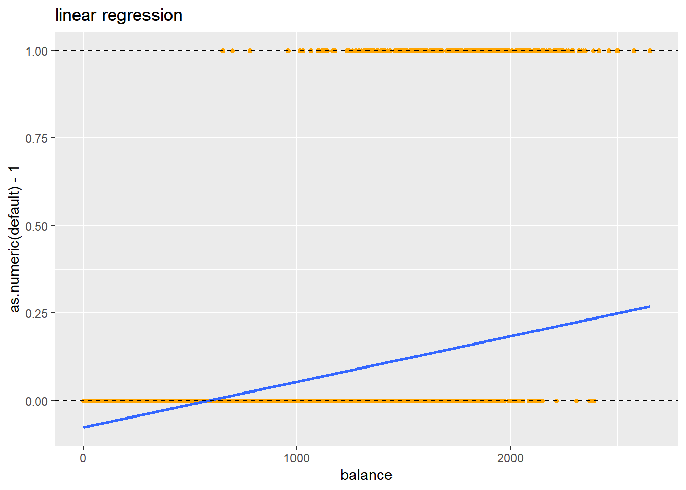
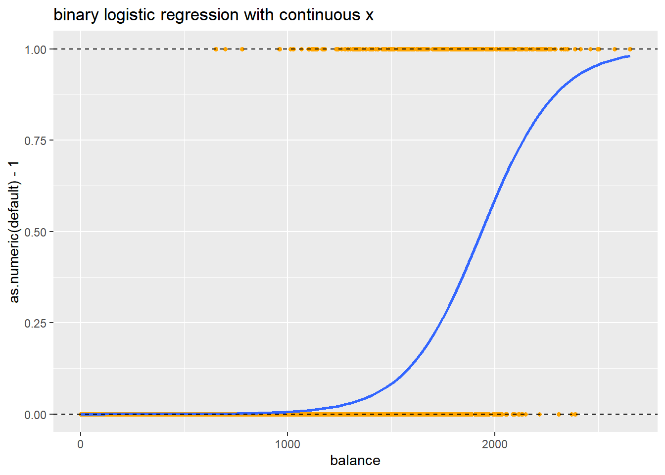
#> # A tibble: 2 × 11 #> term estimate std.error statistic p.value conf.low conf.high z_value #> <chr> <dbl> <dbl> <dbl> <dbl> <dbl> <dbl> <dbl> #> 1 (Intercept) -10.7 0.361 -29.5 3.62e-191 -1.14e+1 -9.97 -29.5 #> 2 balance 0.00550 0.000220 25.0 1.98e-137 5.08e-3 0.00594 25.0 #> # ℹ 3 more variables: Wald_ChiSquare <dbl>, OR <dbl>, `OR 95% CI` <chr> ggplot ( df ,aes ( balance ,as.numeric ( default ) - 1 ) ) + geom_point ( color= "orange" ,size= 1.25 ) +
geom_smooth ( method = "glm" ,
method.args= list ( family= binomial ( link = "logit" ) ) ,se= FALSE ) +
geom_hline ( yintercept = c ( 0 ,1 ) ,linetype= 2 ) +
ggtitle ( "binary logistic regression with continuous x" )
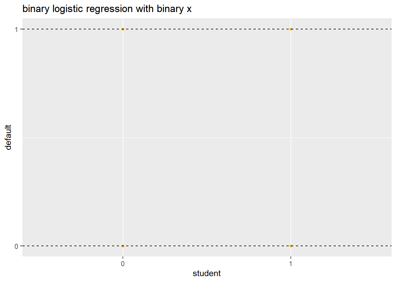
Show the code logit_binary_x <- logit_spec %>% fit ( default ~ student , data = df ) tidy ( logit_binary_x ) #> # A tibble: 2 × 5 #> term estimate std.error statistic p.value #> <chr> <dbl> <dbl> <dbl> <dbl> #> 1 (Intercept) -3.50 0.0707 -49.6 0 #> 2 student1 0.405 0.115 3.52 0.000431 ggplot ( df ,aes ( student ,as.numeric ( default ) - 1 ) ) + geom_point ( color= "orange" ,size= 1.25 ) +
geom_smooth ( method = "glm" ,
method.args= list ( family= binomial ( link = "logit" ) ) ,se= FALSE ) +
geom_hline ( yintercept = c ( 0 ,1 ) ,linetype= 2 ) +
scale_y_continuous ( "default" , breaks = c ( 0 ,1 ) ) +
ggtitle ( "binary logistic regression with binary x" )
二分类多元逻辑回归
当\(K=2\) 时,\(k=l=1,p>1\) 即多元逻辑回归(multiple logistic regression)。
优势(odds)
\[
Odds=\frac{\pi(X)}{1-\pi(X)}=e^{\beta_0+\beta_1X_1+\beta_2X_2+...+\beta_pX_p}
\]
log odds (logit)
\[
logit(\pi(X))=\ln (\frac{\pi(X)}{1-\pi(X)})=\beta_0+\beta_1X_1+\beta_2X_2+...+\beta_pX_p
\]
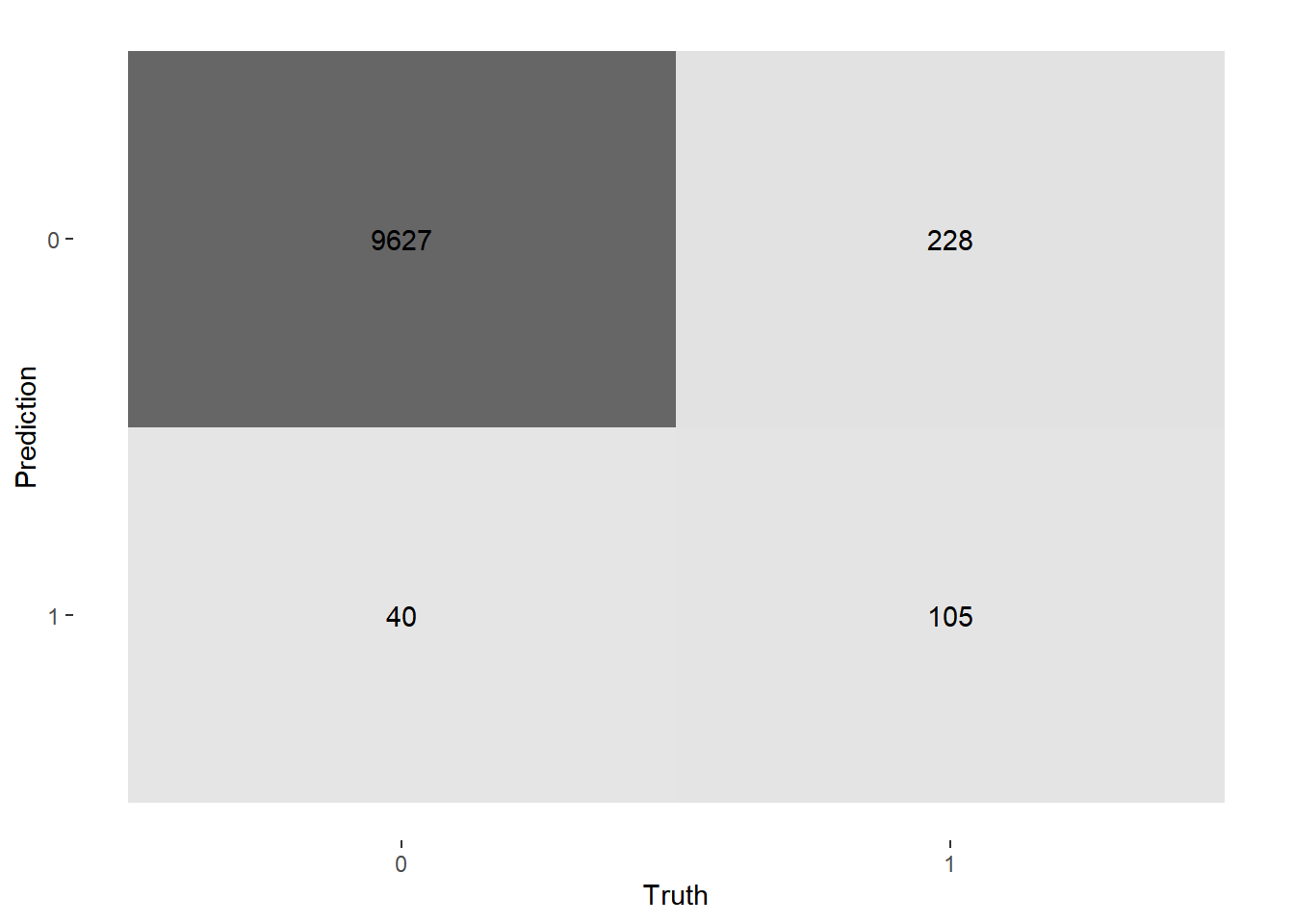
Show the code logit_multiple <- logit_spec %>% fit ( default ~ balance + income + student ,data= df ) tidy ( logit_multiple ) #> # A tibble: 4 × 5 #> term estimate std.error statistic p.value #> <chr> <dbl> <dbl> <dbl> <dbl> #> 1 (Intercept) -10.9 0.492 -22.1 4.91e-108 #> 2 balance 0.00574 0.000232 24.7 4.22e-135 #> 3 income 0.00000303 0.00000820 0.370 7.12e- 1 #> 4 student1 -0.647 0.236 -2.74 6.19e- 3 # confusion matrix 混淆矩阵 augment ( logit_multiple , new_data = df ) %>% conf_mat ( truth = default , estimate = .pred_class ) %>%
autoplot ( type = "heatmap" ) Show the code #准确性 ( 9627 + 105 ) / ( 9627 + 105 + 40 + 228 ) #> [1] 0.9732 augment ( logit_multiple , new_data = df ) %>% accuracy ( truth = default , estimate = .pred_class )
#> # A tibble: 1 × 3 #> .metric .estimator .estimate #> <chr> <chr> <dbl> #> 1 accuracy binary 0.973
Show the code df_new <- tibble ( balance = c ( 1000 , 2000 ) ,
income = c ( 14144 ,24141 ) ,
student = factor ( c ( 1 , 0 ) ) ,)
predict ( logit_multiple , new_data = df_new ,type= "class" ) #> # A tibble: 2 × 1 #> .pred_class #> <fct> #> 1 0 #> 2 1 predict ( logit_multiple , new_data = df_new , type = "prob" ) #> # A tibble: 2 × 2 #> .pred_0 .pred_1 #> <dbl> <dbl> #> 1 0.997 0.00322 #> 2 0.337 0.663
似然比检验
likelihood ratio tests (LRT)
比较两个嵌套模型,log-likelihood (logLL)
相应的p-value 源自具有 个自由度的 卡方 分布(即模型中测试的参数数量之差)。
Show the code logit_binary_y #> parsnip model object #> #> #> Call: stats::glm(formula = default ~ balance, family = ~binomial(link = "logit"), #> data = data) #> #> Coefficients: #> (Intercept) balance #> -10.651331 0.005499 #> #> Degrees of Freedom: 9999 Total (i.e. Null); 9998 Residual #> Null Deviance: 2921 #> Residual Deviance: 1596 AIC: 1600 logit_multiple #> parsnip model object #> #> #> Call: stats::glm(formula = default ~ balance + income + student, family = ~binomial(link = "logit"), #> data = data) #> #> Coefficients: #> (Intercept) balance income student1 #> -1.087e+01 5.737e-03 3.033e-06 -6.468e-01 #> #> Degrees of Freedom: 9999 Total (i.e. Null); 9996 Residual #> Null Deviance: 2921 #> Residual Deviance: 1572 AIC: 1580 LRT = 2 * ( logLik ( logit_multiple $ fit ) - logLik ( logit_binary_y $ fit ) ) LRT #> 'log Lik.' 24.90686 (df=4) pval = 1 - pchisq ( LRT ,2 ) pval #> 'log Lik.' 3.904316e-06 (df=4) out <- anova ( logit_binary_y $ fit , logit_multiple $ fit ) out #> Analysis of Deviance Table #> #> Model 1: default ~ balance #> Model 2: default ~ balance + income + student #> Resid. Df Resid. Dev Df Deviance Pr(>Chi) #> 1 9998 1596.5 #> 2 9996 1571.5 2 24.907 3.904e-06 *** #> --- #> Signif. codes: 0 '***' 0.001 '**' 0.01 '*' 0.05 '.' 0.1 ' ' 1 1 - pchisq ( out $ Deviance [ 2 ] ,2 ) #> [1] 3.904316e-06
K>2 多分类逻辑回归
用于处理具有多于两个类别的响应变量的情况。例如,分类问题中的三个或更多类别。
当\(K>2\) 时,\(k,l,p>1\) 即多项逻辑回归(multinomial logistic regression)。
\[
\ln (\frac{P(Y=k|X=x)}{P(Y=K|X=x)})=\beta_{k0}+\beta_{k1}X_1+\beta_{k2}X_2+...+\beta_{kp}X_p
\]
nnet::multinom()
Show the code mn_spec <- multinom_reg ( mode = "classification" , engine = "nnet" ) iris_mnlogit <- mn_spec %>% fit ( Species ~ . , data = iris )
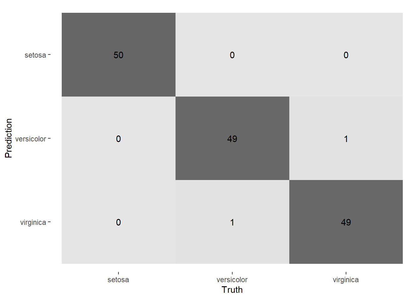
iris_mnlogit %>% glance ( ) #> # A tibble: 1 × 4 #> edf deviance AIC nobs #> <dbl> <dbl> <dbl> <int> #> 1 10 11.9 31.9 150 iris_mnlogit %>% tidy ( ) #> # A tibble: 10 × 6 #> y.level term estimate std.error statistic p.value #> <chr> <chr> <dbl> <dbl> <dbl> <dbl> #> 1 versicolor (Intercept) 18.7 35.0 0.534 0.593 #> 2 versicolor Sepal.Length -5.46 89.9 -0.0607 0.952 #> 3 versicolor Sepal.Width -8.71 157. -0.0554 0.956 #> 4 versicolor Petal.Length 14.2 60.2 0.237 0.813 #> 5 versicolor Petal.Width -3.10 45.5 -0.0681 0.946 #> 6 virginica (Intercept) -23.8 35.8 -0.666 0.505 #> 7 virginica Sepal.Length -7.92 89.9 -0.0881 0.930 #> 8 virginica Sepal.Width -15.4 157. -0.0978 0.922 #> 9 virginica Petal.Length 23.7 60.5 0.391 0.696 #> 10 virginica Petal.Width 15.1 45.9 0.330 0.742 augment ( iris_mnlogit , new_data = iris ) %>% conf_mat ( truth = Species , estimate = .pred_class ) %>%
autoplot ( type = "heatmap" )
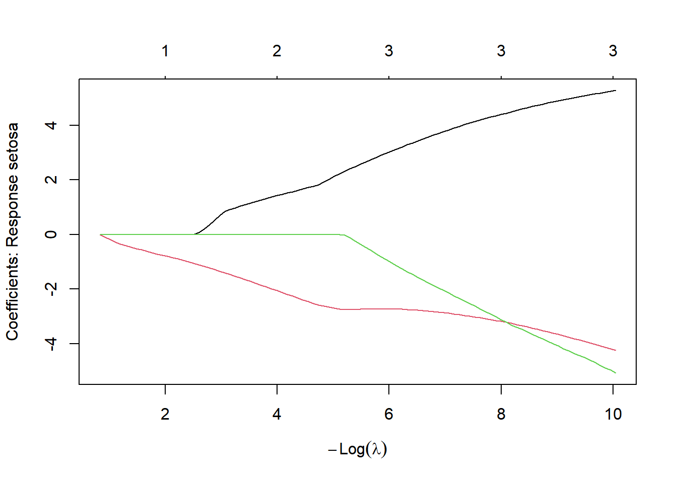
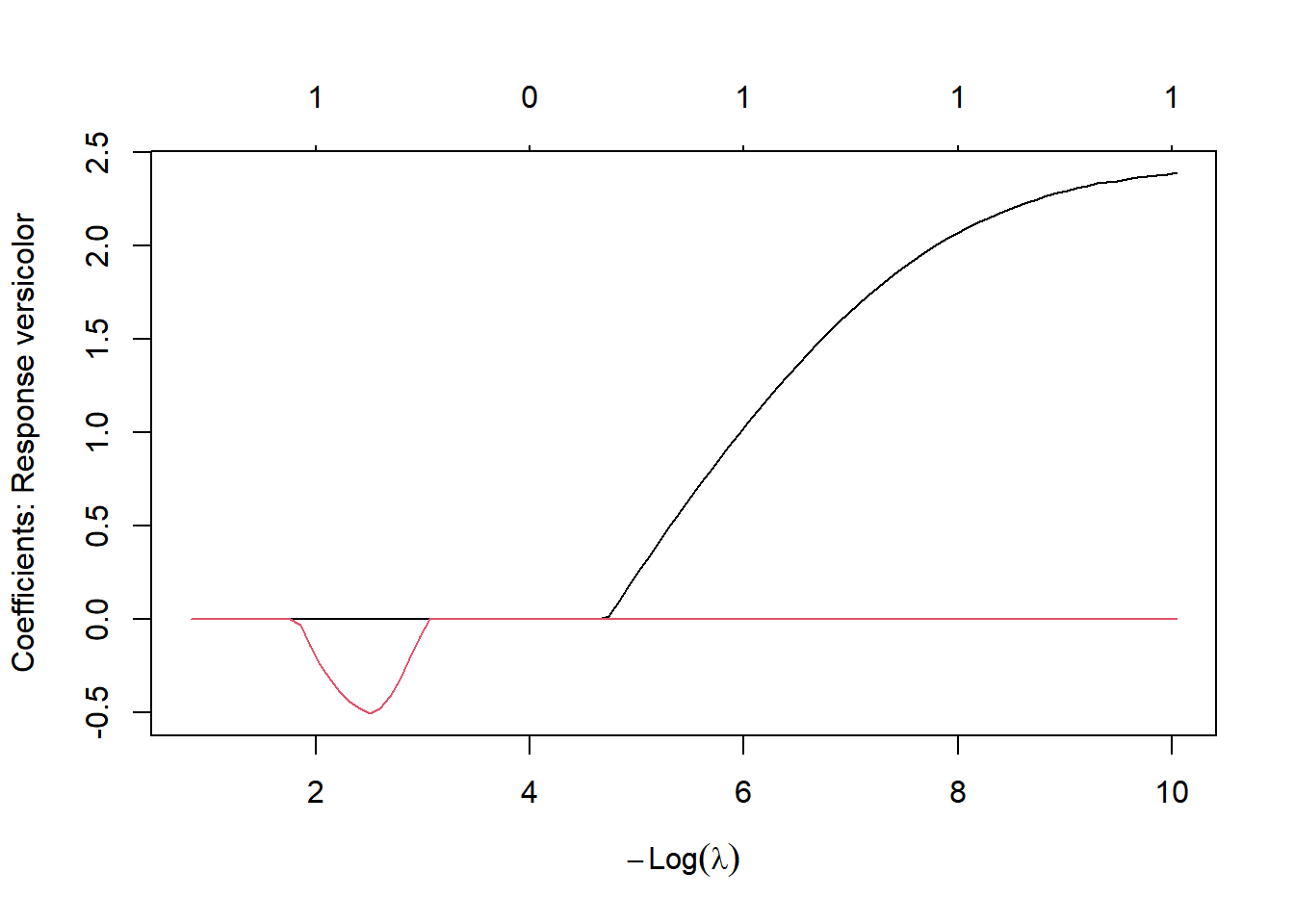
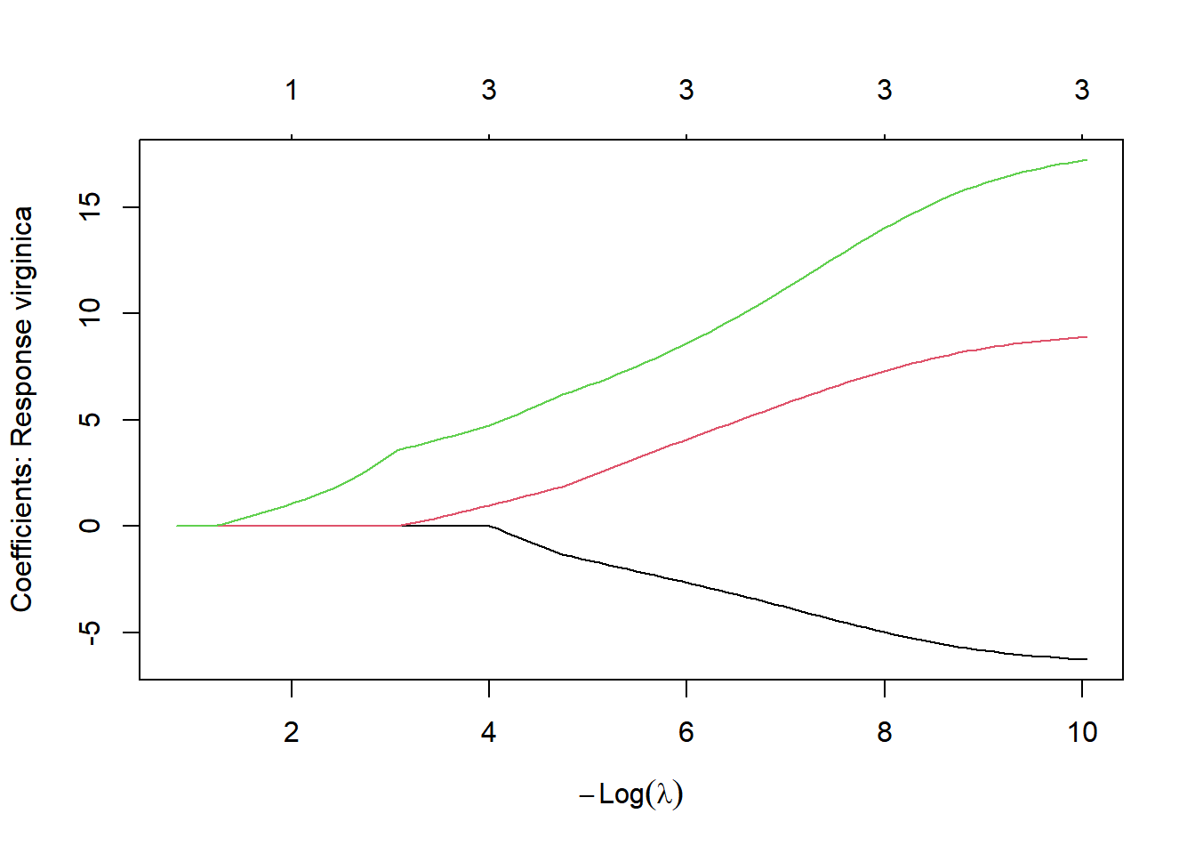
glmnet::glmnet()
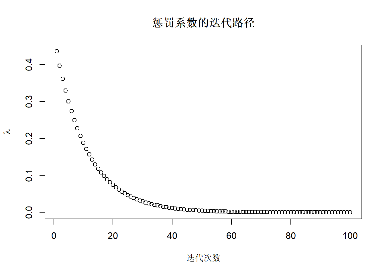
Show the code library ( glmnet ) # 多项回归 iris_glmnet <- glmnet ( x = iris [ , - 5 ] , y = iris [ , 5 ] , family = "multinomial" ) iris_glmnet #> #> Call: glmnet(x = iris[, -5], y = iris[, 5], family = "multinomial") #> #> Df %Dev Lambda #> 1 0 0.00 0.43500 #> 2 1 6.56 0.39640 #> 3 1 12.05 0.36110 #> 4 1 16.73 0.32910 #> 5 1 20.78 0.29980 #> 6 2 25.37 0.27320 #> 7 2 29.66 0.24890 #> 8 2 33.54 0.22680 #> 9 2 37.10 0.20670 #> 10 2 40.40 0.18830 #> 11 2 43.47 0.17160 #> 12 3 46.47 0.15630 #> 13 3 49.57 0.14240 #> 14 3 52.38 0.12980 #> 15 3 54.97 0.11830 #> 16 3 57.36 0.10780 #> 17 3 59.60 0.09818 #> 18 3 61.71 0.08946 #> 19 3 63.72 0.08151 #> 20 3 65.70 0.07427 #> 21 3 67.65 0.06767 #> 22 3 69.54 0.06166 #> 23 3 71.38 0.05618 #> 24 3 73.12 0.05119 #> 25 3 74.71 0.04664 #> 26 3 76.24 0.04250 #> 27 3 77.67 0.03872 #> 28 3 78.99 0.03528 #> 29 3 80.21 0.03215 #> 30 3 81.33 0.02929 #> 31 3 82.36 0.02669 #> 32 3 83.31 0.02432 #> 33 3 84.18 0.02216 #> 34 3 84.99 0.02019 #> 35 3 85.73 0.01840 #> 36 3 86.53 0.01676 #> 37 3 87.34 0.01527 #> 38 3 88.06 0.01392 #> 39 3 88.73 0.01268 #> 40 3 89.34 0.01155 #> 41 3 89.89 0.01053 #> 42 3 90.40 0.00959 #> 43 4 90.87 0.00874 #> 44 4 91.34 0.00796 #> 45 4 91.77 0.00726 #> 46 4 92.16 0.00661 #> 47 4 92.52 0.00602 #> 48 4 92.85 0.00549 #> 49 4 93.16 0.00500 #> 50 4 93.44 0.00456 #> 51 4 93.69 0.00415 #> 52 4 93.92 0.00378 #> 53 4 94.14 0.00345 #> 54 4 94.34 0.00314 #> 55 4 94.52 0.00286 #> 56 4 94.68 0.00261 #> 57 4 94.83 0.00238 #> 58 4 94.97 0.00216 #> 59 4 95.10 0.00197 #> 60 4 95.22 0.00180 #> 61 4 95.33 0.00164 #> 62 4 95.43 0.00149 #> 63 4 95.52 0.00136 #> 64 4 95.60 0.00124 #> 65 4 95.68 0.00113 #> 66 4 95.75 0.00103 #> 67 4 95.81 0.00094 #> 68 4 95.87 0.00085 #> 69 4 95.92 0.00078 #> 70 4 95.97 0.00071 #> 71 4 96.01 0.00065 #> 72 4 96.05 0.00059 #> 73 4 96.09 0.00054 #> 74 4 96.12 0.00049 #> 75 4 96.15 0.00045 #> 76 4 96.18 0.00041 #> 77 4 96.20 0.00037 #> 78 4 96.22 0.00034 #> 79 4 96.24 0.00031 #> 80 4 96.26 0.00028 #> 81 4 96.27 0.00025 #> 82 4 96.29 0.00023 #> 83 4 96.30 0.00021 #> 84 4 96.31 0.00019 #> 85 4 96.32 0.00018 #> 86 4 96.33 0.00016 #> 87 4 96.33 0.00015 #> 88 4 96.34 0.00013 #> 89 4 96.35 0.00012 #> 90 4 96.35 0.00011 #> 91 4 96.35 0.00010 #> 92 4 96.36 0.00009 #> 93 4 96.36 0.00008 #> 94 4 96.36 0.00008 #> 95 4 96.37 0.00007 #> 96 4 96.37 0.00006 #> 97 4 96.37 0.00006 #> 98 4 96.37 0.00005 #> 99 4 96.38 0.00005 #> 100 4 96.38 0.00004 summary ( iris_glmnet ) #> Length Class Mode #> a0 300 -none- numeric #> beta 3 -none- list #> dfmat 300 -none- numeric #> df 100 -none- numeric #> dim 2 -none- numeric #> lambda 100 -none- numeric #> dev.ratio 100 -none- numeric #> nulldev 1 -none- numeric #> npasses 1 -none- numeric #> jerr 1 -none- numeric #> offset 1 -none- logical #> classnames 3 -none- character #> grouped 1 -none- logical #> call 4 -none- call #> nobs 1 -none- numeric plot ( iris_glmnet ) Show the code plot ( iris_glmnet $ lambda , ylab = expression ( lambda ) , xlab = "迭代次数" , main = "惩罚系数的迭代路径"
) Show the code # 选择一个迭代趋于稳定时的 lambda,比如 iris_glmnet$lambda[80] coef ( iris_glmnet , s = 0.0002796185 ) #> $setosa #> 5 x 1 sparse Matrix of class "dgCMatrix" #> s=0.0002796185 #> (Intercept) 17.015429 #> Sepal.Length . #> Sepal.Width 4.486992 #> Petal.Length -3.250342 #> Petal.Width -3.315393 #> #> $versicolor #> 5 x 1 sparse Matrix of class "dgCMatrix" #> s=0.0002796185 #> (Intercept) 8.132656 #> Sepal.Length 2.123980 #> Sepal.Width . #> Petal.Length . #> Petal.Width . #> #> $virginica #> 5 x 1 sparse Matrix of class "dgCMatrix" #> s=0.0002796185 #> (Intercept) -25.148085 #> Sepal.Length . #> Sepal.Width -5.176029 #> Petal.Length 7.536940 #> Petal.Width 14.481524 iris_pred_glmnet <- predict ( object = iris_glmnet , newx = as.matrix ( iris [ , - 5 ] ) ,
s = 0.0002796185 , type = "class"
)
Show the code mn_spec <- multinom_reg ( mode = "classification" , engine = "glmnet" , penalty = 0 )
iris_mnlogit <- mn_spec %>% fit ( Species ~ . , data = iris )
iris_mnlogit %>% glance ( ) #> # A tibble: 1 × 3 #> nulldev npasses nobs #> <dbl> <int> <int> #> 1 330. 6546 150 iris_mnlogit $ fit %>% tidy ( ) %>% DT :: datatable ( )
有序逻辑回归
\[
\ln \left(\frac{P(Y\le k|X=x)}{1-P(Y\le k|X=x)}\right)
\]
Show the code # 数据集 icpsr acl <- read_rds ( "data/advanced_acl_data.rds" ) acl $ PhysActCat_W1 <- factor ( acl $ PhysActCat_W1 ,ordered = T ) str ( acl $ PhysActCat_W1 ) #> Ord.factor w/ 5 levels "(1) Low_5th"<..: 1 3 5 3 2 2 3 1 4 5 ... ordered_logit <- MASS :: polr ( PhysActCat_W1 ~ SelfEfficacy_W1 , data = acl , method = "logistic" )
ordered_logit %>% summary ( ) #> Call: #> MASS::polr(formula = PhysActCat_W1 ~ SelfEfficacy_W1, data = acl, #> method = "logistic") #> #> Coefficients: #> Value Std. Error t value #> SelfEfficacy_W1 0.2431 0.02893 8.404 #> #> Intercepts: #> Value Std. Error t value #> (1) Low_5th|(2) 2Low_5th -0.9332 0.0371 -25.1533 #> (2) 2Low_5th|(3) 3Low_5th -0.2688 0.0338 -7.9606 #> (3) 3Low_5th|(4) 4Low_5th 0.8470 0.0364 23.2527 #> (4) 4Low_5th|(5) Hi_5th 1.5298 0.0435 35.1647 #> #> Residual Deviance: 11196.86 #> AIC: 11206.86 predict ( ordered_logit ,acl ,type = "prob" ) %>% as_tibble ( ) %>%
DT :: datatable ( ) Show the code
泊松回归
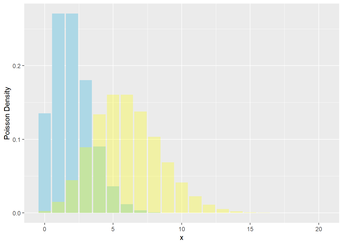
泊松回归用于计数数据,假设响应变量服从泊松分布,并使用对数链接函数(log link function),z-statistic
family=poisson(link = "log")
family = quasipoisson(link = "log"))
\[
P(X=x;\lambda)=\frac{e^{-\lambda}\lambda ^x}{x!}
\]
Show the code # 泊松回归模型 pois_spec <- poisson_reg ( ) %>% set_mode ( "regression" ) %>%
set_engine ( "glm" ,family= poisson ( link = "log" ) )
pois_rec_spec <- recipe ( bikers ~ mnth + hr + workingday + temp + weathersit , data = df2 ) %>% step_dummy ( all_nominal_predictors ( ) ) # 虚拟变量
pois_wf <- workflow ( ) %>% add_recipe ( pois_rec_spec ) %>%
add_model ( pois_spec )
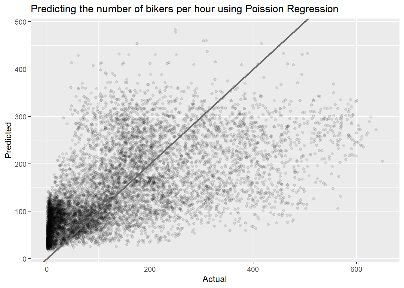
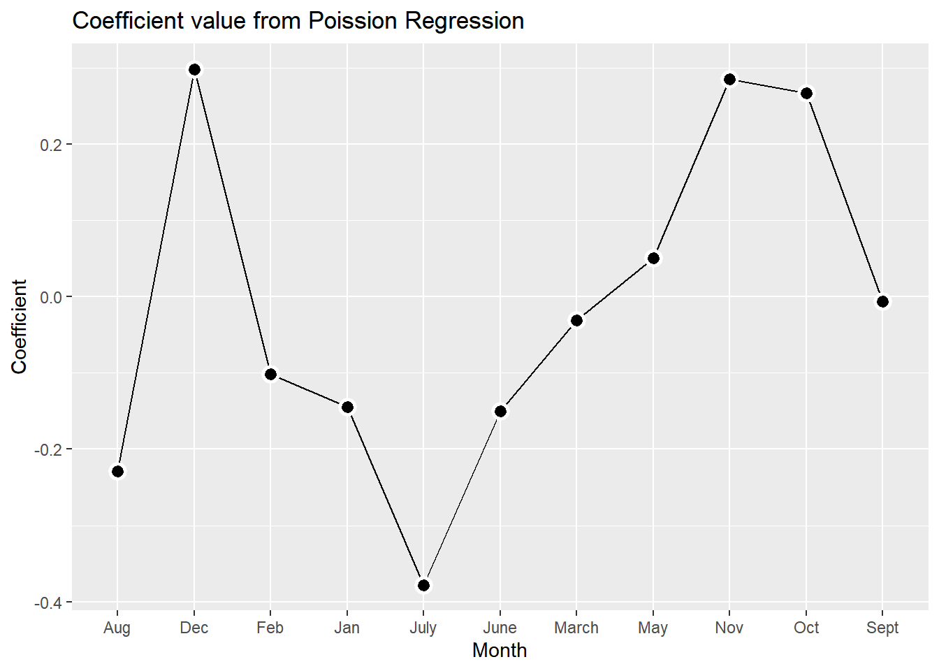
pois_fit <- pois_wf %>% fit ( data = df2 ) tidy ( pois_fit ) #> # A tibble: 18 × 5 #> term estimate std.error statistic p.value #> <chr> <dbl> <dbl> <dbl> <dbl> #> 1 (Intercept) 3.01 0.00632 477. 0 #> 2 hr 0.0507 0.000144 352. 0 #> 3 workingday -0.0128 0.00195 -6.57 4.91e- 11 #> 4 temp 2.56 0.00995 258. 0 #> 5 mnth_Aug -0.229 0.00470 -48.7 0 #> 6 mnth_Dec 0.298 0.00501 59.5 0 #> 7 mnth_Feb -0.102 0.00592 -17.2 5.28e- 66 #> 8 mnth_Jan -0.145 0.00678 -21.4 1.74e-101 #> 9 mnth_July -0.378 0.00496 -76.2 0 #> 10 mnth_June -0.150 0.00462 -32.5 1.32e-231 #> 11 mnth_March -0.0312 0.00534 -5.83 5.44e- 9 #> 12 mnth_May 0.0508 0.00434 11.7 1.43e- 31 #> 13 mnth_Nov 0.285 0.00461 61.8 0 #> 14 mnth_Oct 0.267 0.00432 61.7 0 #> 15 mnth_Sept -0.00653 0.00443 -1.47 1.41e- 1 #> 16 weathersit_cloudy.misty -0.0308 0.00216 -14.2 5.70e- 46 #> 17 weathersit_heavy.rain.snow -0.646 0.167 -3.87 1.08e- 4 #> 18 weathersit_light.rain.snow -0.473 0.00404 -117. 0 # 绘制实际值与预测值的关系图 augment ( pois_fit , new_data = df2 , type = "response" ) %>% ggplot ( aes ( bikers , .pred ) ) +
geom_point ( alpha = 0.1 ) +
geom_abline ( slope = 1 ,
linewidth = 1 ,
color = "grey40" ) +
labs ( title = "Predicting the number of bikers per hour using Poission Regression" , x = "Actual" , y = "Predicted" )
Show the code pois_fit_coef_mnths <- tidy ( pois_fit ) %>%
dplyr :: filter ( grepl ( "^mnth" , term ) ) %>%
mutate (
term = stringr :: str_replace ( term , "mnth_" , "" ) ,
term = forcats :: fct_inorder ( term )
)
pois_fit_coef_mnths %>% ggplot ( aes ( term , estimate ) ) +
geom_line ( group = 1 ,na.rm = TRUE ) +
geom_point ( shape = 21 , size = 3 , stroke = 1.5 ,
fill = "black" , color = "white" ,na.rm = TRUE ) +
labs ( title = "Coefficient value from Poission Regression" ,
x = "Month" , y = "Coefficient" )
Show the code pois_acl <- pois_spec %>% fit ( NChronic12_W1 ~ SelfEfficacy_W1 ,data = acl )
pois_acl %>% glance ( ) #> # A tibble: 1 × 8 #> null.deviance df.null logLik AIC BIC deviance df.residual nobs #> <dbl> <int> <dbl> <dbl> <dbl> <dbl> <int> <int> #> 1 5217. 3616 -5161. 10327. 10339. 5114. 3615 3617 pois_acl %>% tidy ( ) #> # A tibble: 2 × 5 #> term estimate std.error statistic p.value #> <chr> <dbl> <dbl> <dbl> <dbl> #> 1 (Intercept) 0.0713 0.0162 4.40 1.06e- 5 #> 2 SelfEfficacy_W1 -0.150 0.0144 -10.4 3.97e-25 AIC ( pois_acl $ fit ) #> [1] 10326.52 BIC ( pois_acl $ fit ) #> [1] 10338.9
负二项回归
负二项回归用于处理计数数据且存在过度离散(overdispersion)的问题即当均值不等于方差。
log link function,z-statistic
probability mass function :
\[
P(X=x;\lambda,\nu)=\binom{x+\nu - 1}{ x} \left ( \frac{\lambda}{\lambda +\nu} \right)^x \left ( \frac{\nu}{\nu + \lambda} \right)^{\nu}
\]
负二项分布的均值是 \(\lambda\) ,
方差是 \(\lambda + \frac{\lambda ^2}{\nu}\) 。
Show the code library ( MASS ) # 负二项回归模型 nb_spec <- linear_reg ( ) %>% set_engine ( "glm" , family = MASS :: negative.binomial ( theta = 1 , link = "log" ) )
nb_acl <- nb_spec %>% fit ( NChronic12_W1 ~ SelfEfficacy_W1 , data = acl )
# 查看模型结果 nb_acl %>% glance ( ) #> # A tibble: 1 × 8 #> null.deviance df.null logLik AIC BIC deviance df.residual nobs #> <dbl> <int> <dbl> <dbl> <dbl> <dbl> <int> <int> #> 1 2946. 3616 -5220. 10443. 10456. 2898. 3615 3617 nb_acl %>% tidy ( ) #> # A tibble: 2 × 5 #> term estimate std.error statistic p.value #> <chr> <dbl> <dbl> <dbl> <dbl> #> 1 (Intercept) 0.0715 0.0181 3.95 8.10e- 5 #> 2 SelfEfficacy_W1 -0.148 0.0169 -8.75 3.18e-18 AIC ( nb_acl $ fit ) #> [1] 10443.43 BIC ( nb_acl $ fit ) #> [1] 10455.82 # MASS::glm.nb()
零膨胀模型(zero-inflated)
逻辑回归+以上之一
正则化广义线性模型
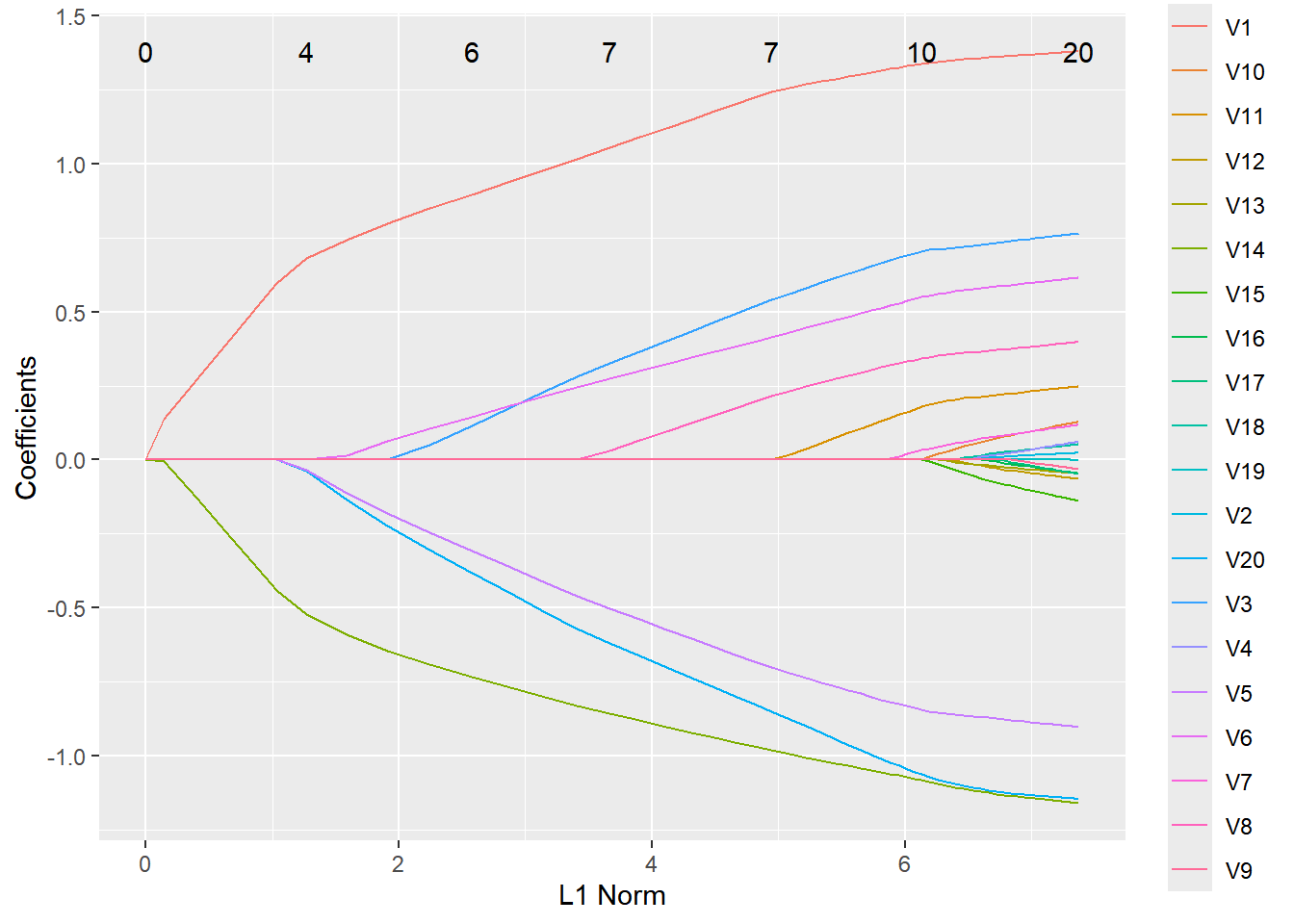
Ridge、Lasso
Show the code
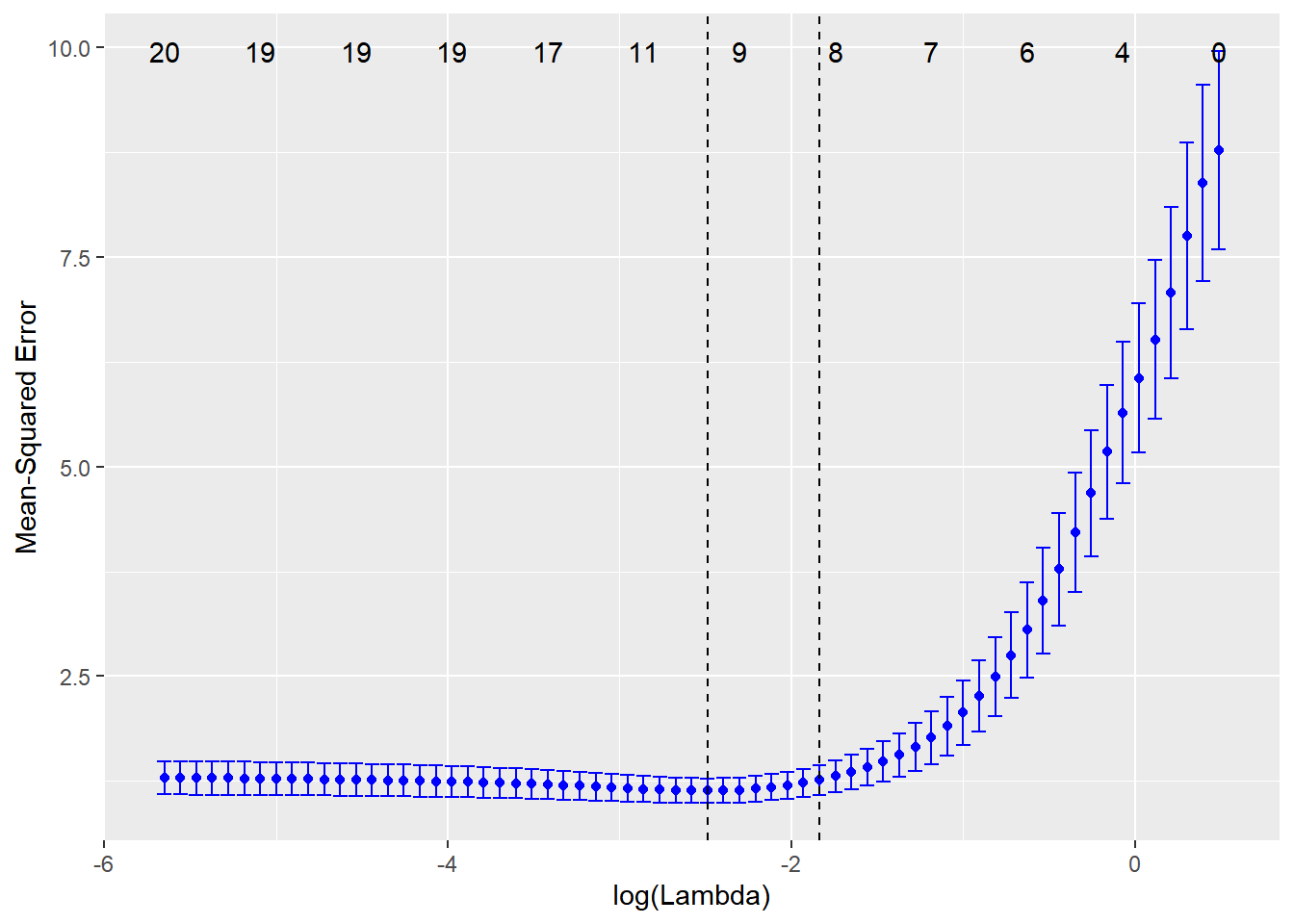
Show the code fit <- glmnet :: cv.glmnet ( x = QuickStartExample $ x , y = QuickStartExample $ y ) autoplot ( fit , colour = 'blue' )