12 简单线性回归
12.1 模型表达
简单线性回归用于解释一个数值变量(因变量)和一个自变量之间的线性关系。模型形式一般为:
\[ Y=X\beta + \epsilon \]
其中, Y 是因变量,X 是自变量矩阵,β 是回归系数,ϵ 是误差项。
\[ Y_i=\beta_0+ \beta_1 X_i+\epsilon_i,其中\epsilon_i\sim N(0,\sigma^2) \]
Show the code
lm_tv <- lm(sales ~ TV, data = advertising)
# 模型摘要
summary(lm_tv)
#>
#> Call:
#> lm(formula = sales ~ TV, data = advertising)
#>
#> Residuals:
#>     Min      1Q  Median      3Q     Max
#> -8.3860 -1.9545 -0.1913  2.0671  7.2124
#>
#> Coefficients:
#>             Estimate Std. Error t value Pr(>|t|)
#> (Intercept) 7.032594   0.457843   15.36   <2e-16 ***
#> TV          0.047537   0.002691   17.67   <2e-16 ***
#> ---
#> Signif. codes:  0 '***' 0.001 '**' 0.01 '*' 0.05 '.' 0.1 ' ' 1
#>
#> Residual standard error: 3.259 on 198 degrees of freedom
#> Multiple R-squared:  0.6119, Adjusted R-squared:  0.6099
#> F-statistic: 312.1 on 1 and 198 DF,  p-value: < 2.2e-16

parameters::model_parameters(lm_tv)
#> Parameter   | Coefficient |       SE |       95% CI | t(198) |      p
#> ---------------------------------------------------------------------
#> (Intercept) |        7.03 |     0.46 | [6.13, 7.94] |  15.36 | < .001
#> TV          |        0.05 | 2.69e-03 | [0.04, 0.05] |  17.67 | < .001
performance::performance(lm_tv)
#> # Indices of model performance
#>
#> AIC    |   AICc |    BIC |    R2 | R2 (adj.) |  RMSE | Sigma
#> ------------------------------------------------------------
#> 1044.1 | 1044.2 | 1054.0 | 0.612 |     0.610 | 3.242 | 3.259

# 参数估计值、标准误、统计量、p值
broom::tidy(lm_tv, conf.int=T)
#> # A tibble: 2 × 7
#>   term        estimate std.error statistic  p.value conf.low conf.high
#>   <chr>          <dbl>     <dbl>     <dbl>    <dbl>    <dbl>     <dbl>
#> 1 (Intercept)   7.03     0.458        15.4 1.41e-35   6.13      7.94
#> 2 TV            0.0475   0.00269      17.7 1.47e-42   0.0422    0.0528
# 模型统计信息
broom::glance(lm_tv)
#> # A tibble: 1 × 12
#>   r.squared adj.r.squared sigma statistic  p.value    df logLik   AIC   BIC
#>       <dbl>         <dbl> <dbl>     <dbl>    <dbl> <dbl>  <dbl> <dbl> <dbl>
#> 1     0.612         0.610  3.26      312. 1.47e-42     1  -519. 1044. 1054.
#> # ℹ 3 more variables: deviance <dbl>, df.residual <int>, nobs <int>
12.1.1 点须图
Show the code
# 整理回归模型结果
tidy_lm <- tidy(lm_tv, conf.int=T) |>  dplyr::filter(term !='(Intercept)' )
# 绘制点须图
ggplot(tidy_lm, aes(x = estimate, y = term)) +
  geom_point(size = 2, color = "black") + # 绘制点
  geom_errorbar(aes(xmin = conf.low,
                     xmax = conf.high),
                 height = 0, color = "black") + # 绘制误差线
  geom_vline(xintercept = 0, colour = "grey50", linetype = 2) + # 绘制参考线
labs(x = NULL, y = NULL) 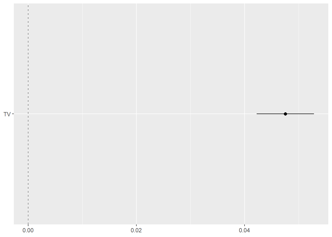
12.1.2 预测
Show the code
# 预测
stats::predict(lm_tv, new_data = advertising) |>
    head(n = 10)
#>         1         2         3         4         5         6         7         8
#> 17.970775  9.147974  7.850224 14.234395 15.627218  7.446162  9.765950 12.746498
#>         9        10
#>  7.441409 16.530414

# 置信区间 平均响应值       取决于方差和样本量     随样本量增加收缩
predict(lm_tv, new_data = advertising, type = "terms") |>
    head(n = 10)
#>            TV
#> 1   3.9482745
#> 2  -4.8745260
#> 3  -6.1722762
#> 4   0.2118946
#> 5   1.6047181
#> 6  -6.5763377
#> 7  -4.2565496
#> 8  -1.2760023
#> 9  -6.5810913
#> 10  2.5079143

# 单个新观测值         主要取决于方差
predict(lm_tv, new_data = advertising, type = "terms") |>
    head(n = 10)
#>            TV
#> 1   3.9482745
#> 2  -4.8745260
#> 3  -6.1722762
#> 4   0.2118946
#> 5   1.6047181
#> 6  -6.5763377
#> 7  -4.2565496
#> 8  -1.2760023
#> 9  -6.5810913
#> 10  2.5079143


# 比较观测值与预测值
augment(lm_tv, new_data = advertising) |>
    head(n = 10)
#> # A tibble: 10 × 8
#>    sales    TV .fitted .resid    .hat .sigma   .cooksd .std.resid
#>    <dbl> <dbl>   <dbl>  <dbl>   <dbl>  <dbl>     <dbl>      <dbl>
#>  1  22.1 230.    18.0   4.13  0.00970   3.25 0.00794       1.27
#>  2  10.4  44.5    9.15  1.25  0.0122    3.27 0.000920      0.387
#>  3   9.3  17.2    7.85  1.45  0.0165    3.27 0.00169       0.449
#>  4  18.5 152.    14.2   4.27  0.00501   3.25 0.00434       1.31
#>  5  12.9 181.    15.6  -2.73  0.00578   3.26 0.00205      -0.839
#>  6   7.2   8.7    7.45 -0.246 0.0180    3.27 0.0000534    -0.0762
#>  7  11.8  57.5    9.77  2.03  0.0105    3.26 0.00208       0.627
#>  8  13.2 120.    12.7   0.454 0.00549   3.27 0.0000538     0.140
#>  9   4.8   8.6    7.44 -2.64  0.0181    3.26 0.00616      -0.818
#> 10  10.6 200.    16.5  -5.93  0.00690   3.24 0.0116       -1.83
predict(lm_tv, new_data = advertising, interval = "confidence") |>
head(n = 10)
predict(lm_tv, new_data = advertising, interval = "prediction") |>
head(n = 10)12.2 模型假设
一般线性模型中,其自变量全部为固定效应自变量,4点假设:
因变量 Y 为连续型数值变量
线性
保证各实测点到回归直线的纵向距离的平方和最小,即使得残差平方和最小。
\[ Q=\sum (Y-\hat Y)^2 \]
Show the code
# 可视化
augment(lm_tv, new_data = advertising) |>
    ggplot(aes(x = TV,y = sales)) +
    geom_linerange(aes(ymin = sales, ymax = .fitted)) +
    geom_point(, color = "red") +
    geom_abline(
        intercept =7.03259,
        slope =  0.04754,
        color = "blue",
        linewidth = 1
    )
残差的正态性 \(\epsilon\sim N(0,\sigma^2)\)
方差齐性 \(Var(ε_i )=σ^2\)
残差的独立性
12.3 模型诊断
Show the code
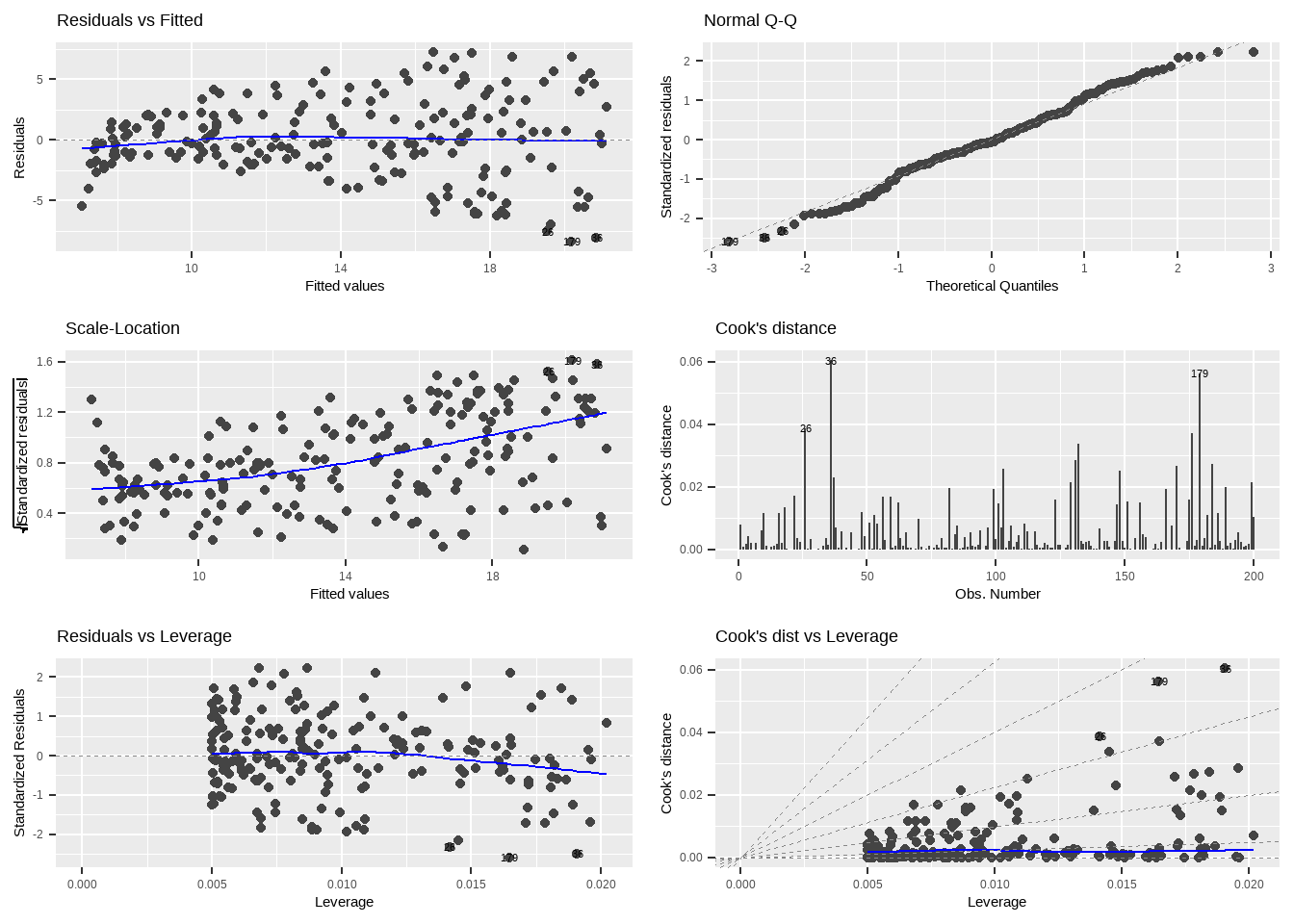
autoplot(lm_tv, which = 1:6, ncol = 2, label.size = 3)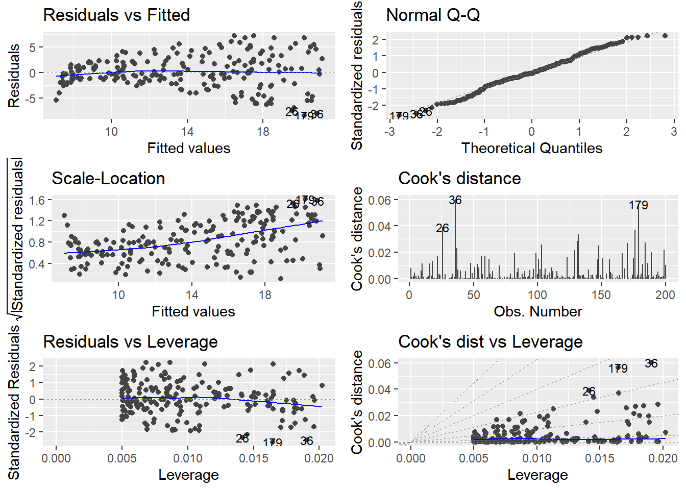
12.3.1 残差图
预测值与残差的关系,线性度,同方差
Show the code
# 检查线性回归模型的残差是否与预测值无关,即残差的分布是否随机。
# 残差应该随机分布在0附近
tibble(
    `Fitted values`=fitted(lm_tv),
    Residuals = residuals(lm_tv)
) |>  ggplot(aes(x = `Fitted values` , y = Residuals)) +
  geom_point(pch=21) +
    geom_smooth(formula = "y~x",color="red",lwd=0.5)+
  geom_hline(yintercept = 0,lty=2) +
  labs(x = "Fitted Values", y = "Residuals")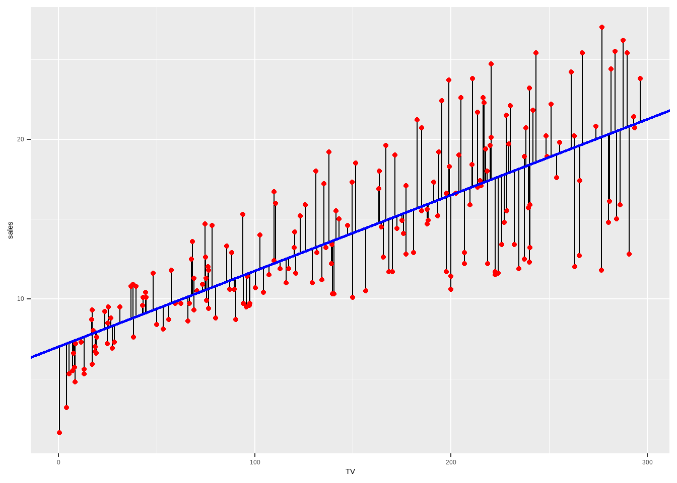
12.3.2 Q-Q图
标准化残差正态性
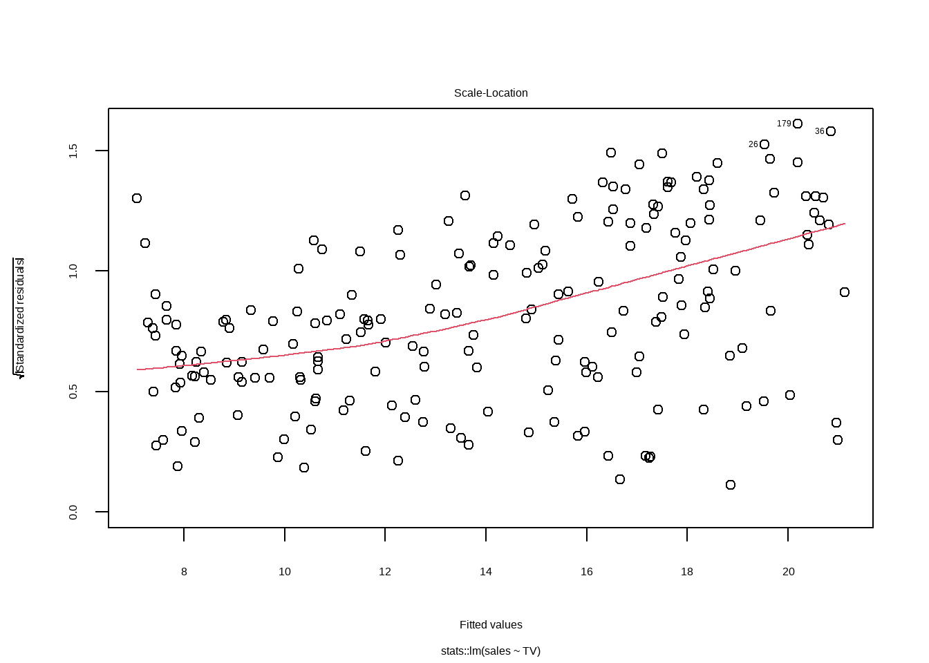
12.3.3 Scale-Location 图
检查同方差性,如果看到漏斗形(残差随着拟合值增大而增大),则可能存在异方差性问题。
标准化残差平方根图
检查残差的正态性,如果看到残差的分布围绕 0 随机散布,没有明显的模式,模型拟合是理想的。
Show the code
plot(lm_tv, which = 3)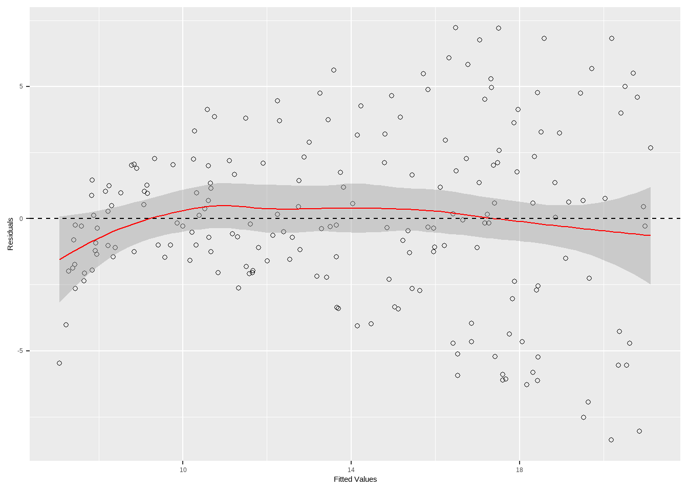
Show the code
# 绘制 Scale-Location 图
tibble(
    fitted_values=fitted(lm_tv),
    StandardizedResiduals = rstudent(lm_tv) ,
) |>
    ggplot(aes(x = fitted_values, y = sqrt(abs(StandardizedResiduals)))) +
    geom_point(pch=21) +
    geom_smooth(color="red",lwd=0.5)+
    labs(title = "Scale-Location Plot",x = "Fitted Values", y = "√|Standardized residuals|")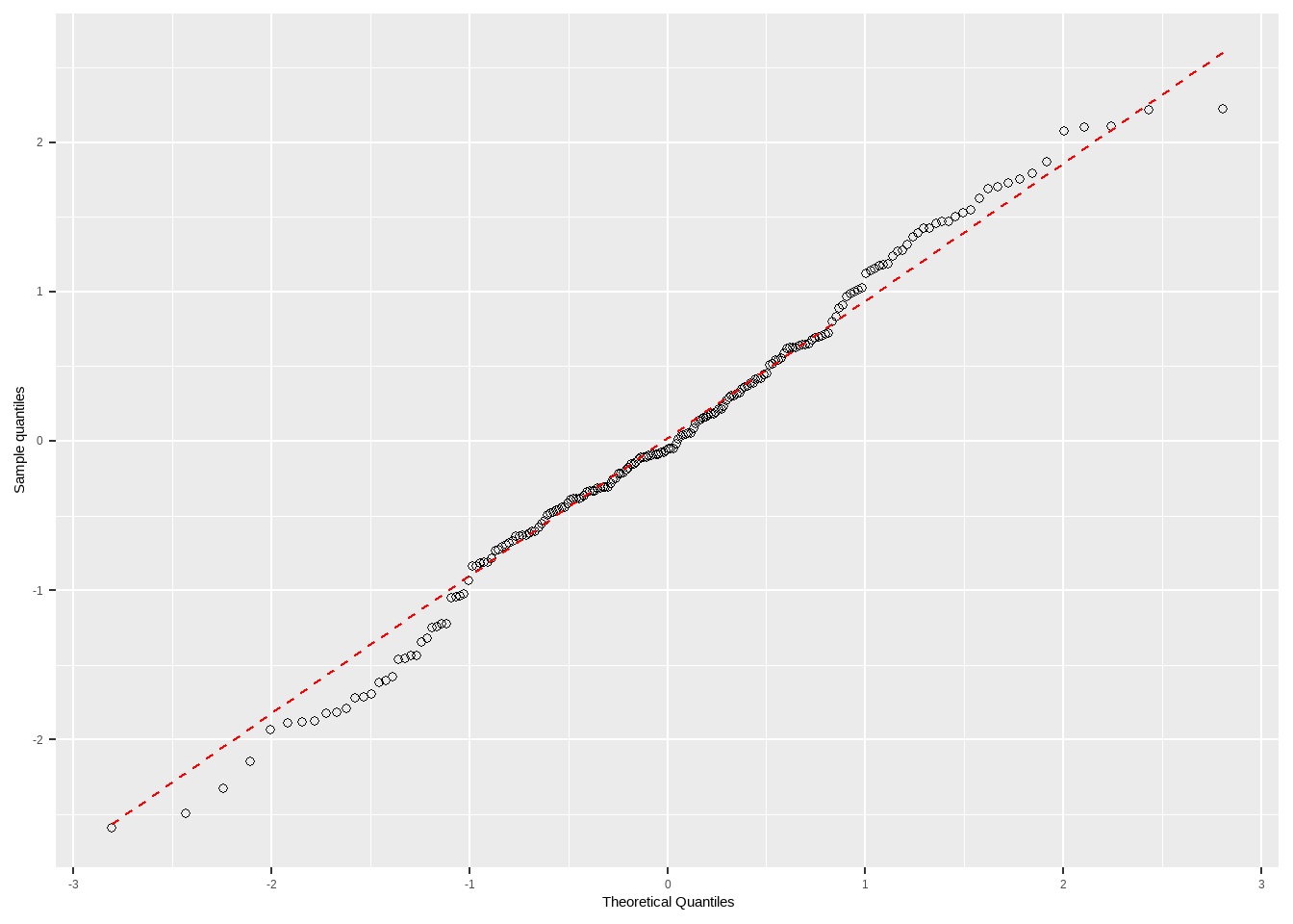
12.3.4 Cook’s距离
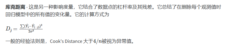
Show the code
Show the code
influence.measures(lmodel)
#> Influence measures of
#>   lm(formula = y ~ x) :
#>
#>     dfb.1_   dfb.x   dffit cov.r  cook.d   hat inf
#> 1  -0.0724 -0.0137 -0.0837 1.431 0.00397 0.103
#> 2  -0.2607  0.1637 -0.2717 1.388 0.03993 0.157
#> 3   0.0822 -0.0555  0.0869 1.554 0.00430 0.169
#> 4   0.2679  0.0174  0.2935 1.178 0.04433 0.100
#> 5   0.1102  0.0548  0.1490 1.408 0.01238 0.116
#> 6  -0.5785  0.1207 -0.5854 0.724 0.13792 0.104
#> 7   0.4851 -0.1676  0.4851 0.925 0.10651 0.114
#> 8  -0.6059  0.3277 -0.6179 0.848 0.16313 0.139
#> 9   0.4957 -0.2572  0.5034 0.996 0.11760 0.135
#> 10  0.0157 -1.0428 -1.1090 9.033 0.68380 0.863   *
Show the code
plot(lm_tv,4) 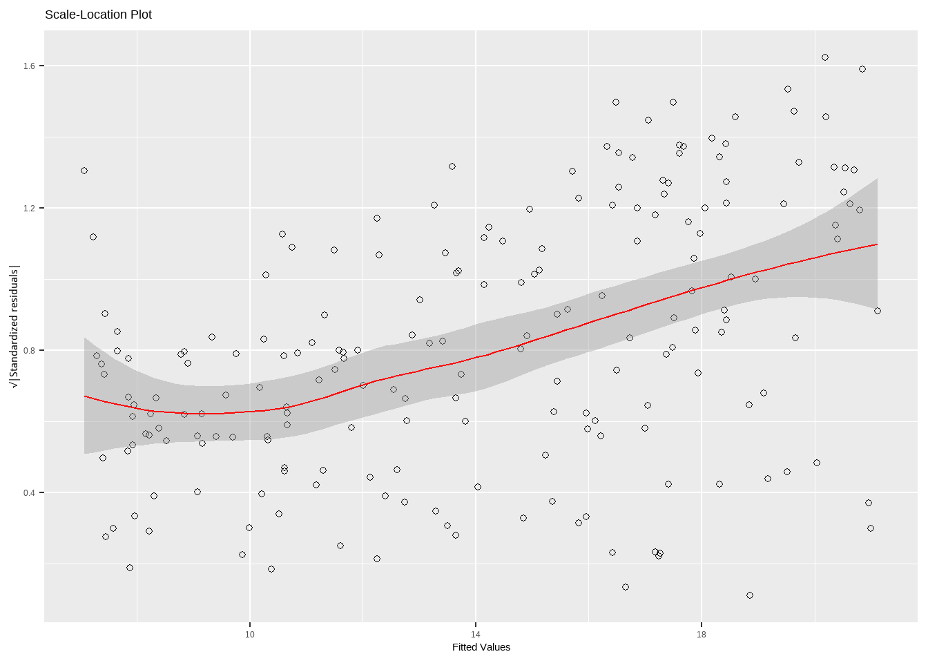
Show the code
threshold <- 4 / (nrow(advertising)-length(lm_tv$coefficients)-2)


tibble(
    x = 1:nrow(advertising),
    cooks_distance = cooks.distance(lm_tv),
    label = factor(if_else(cooks_distance>threshold,x,NA))
) |>
    ggplot() +
    geom_segment(aes(
        x = x,
        xend = x,
        y = 0,
        yend = cooks_distance ,
    )) +
    geom_text(aes(
        x = x,
        y =cooks_distance ,
        label =label,
    ), vjust = -0.2) +
    labs(x = "Observation Index", y = "Cook's Distance")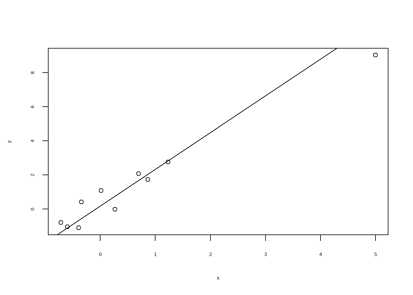
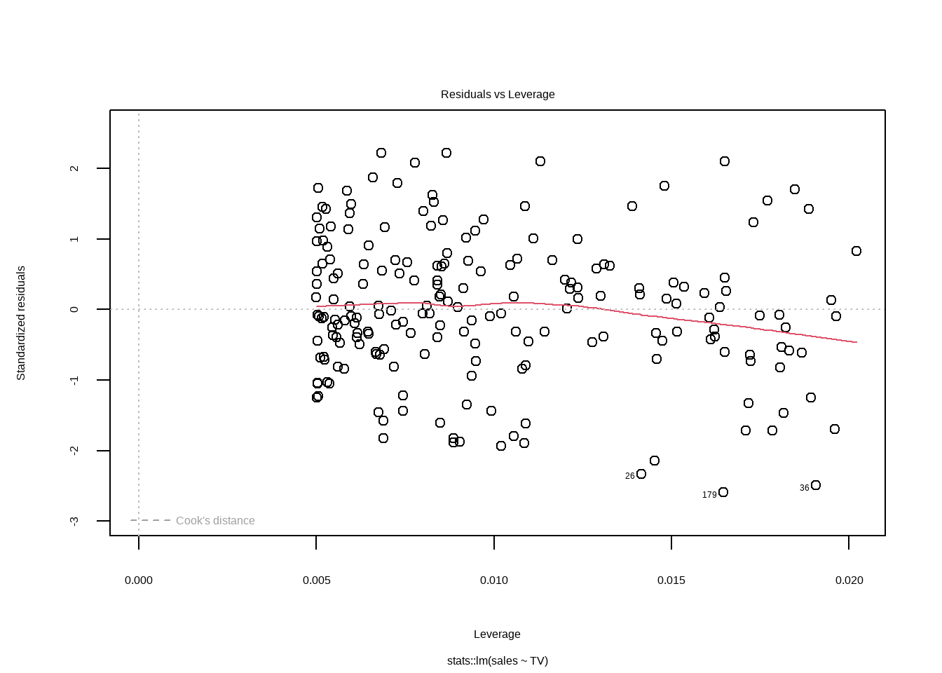
12.3.5 残差-杠杆值图

Show the code
influence(lmodel)$hat     #leverage
#>         1         2         3         4         5         6         7         8
#> 0.1027407 0.1570337 0.1686229 0.1003533 0.1156210 0.1044403 0.1135604 0.1391403
#>         9        10
#> 0.1353478 0.8631394


1/10 + (x-mean(x))^2/(var(x)*9)  #leverage manually computed
#>  [1] 0.1027407 0.1570337 0.1686229 0.1003533 0.1156210 0.1044403 0.1135604
#>  [8] 0.1391403 0.1353478 0.8631394
Show the code
influence(lmodel)$coefficients     #DFBETA
#>     (Intercept)            x
#> 1  -0.015131790 -0.001678535
#> 2  -0.053246101  0.019647712
#> 3   0.017216660 -0.006821716
#> 4   0.053369207  0.002038393
#> 5   0.022861311  0.006672433
#> 6  -0.101915091  0.012493753
#> 7   0.090627673 -0.018400391
#> 8  -0.109982670  0.034951829
#> 9   0.093779788 -0.028593745
#> 10  0.003248704 -0.126864091

dfbeta(lmodel)
#>     (Intercept)            x
#> 1  -0.015131790 -0.001678535
#> 2  -0.053246101  0.019647712
#> 3   0.017216660 -0.006821716
#> 4   0.053369207  0.002038393
#> 5   0.022861311  0.006672433
#> 6  -0.101915091  0.012493753
#> 7   0.090627673 -0.018400391
#> 8  -0.109982670  0.034951829
#> 9   0.093779788 -0.028593745
#> 10  0.003248704 -0.126864091
#computing the DFBETA manually for the 10th observation
coef(lm(y~x)) - coef(lm(y[-10]~x[-10]))
#>  (Intercept)            x
#>  0.003248704 -0.126864091
Show the code
plot(lm_tv,5) 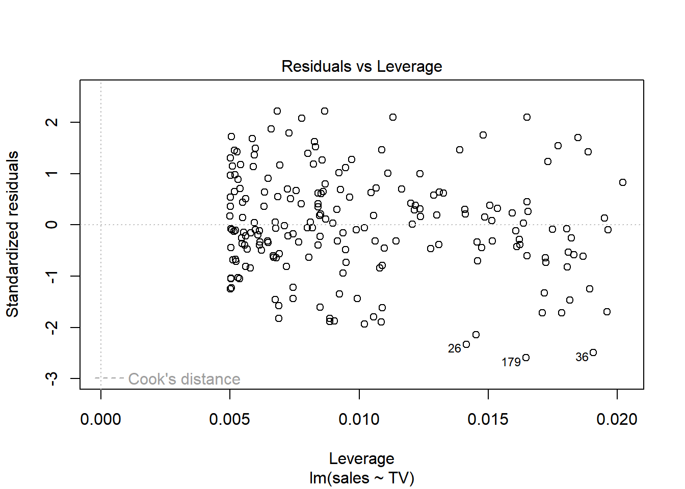
hat 统计量
Show the code
tibble(
    x = 1:nrow(advertising),
    leverage = hatvalues(lm_tv),
    StandardizedResiduals = rstandard(lm_tv) ,
    cooks_distance = cooks.distance(lm_tv),
    label = factor(if_else(cooks_distance>threshold,x,NA))
) |>
    ggplot(aes(x = leverage, y = StandardizedResiduals)) +
    geom_point(pch=21) +
    geom_smooth(color="red",lwd=0.5)+
    scale_x_continuous(limits = c(0, NA)) +
    geom_vline(xintercept = 0, lty = 2) +
    geom_hline(yintercept = 0, lty = 2) +
    ggrepel::geom_text_repel(mapping = aes(label = label))+
    labs(x = "Leverage Values", y = "Standardized residuals")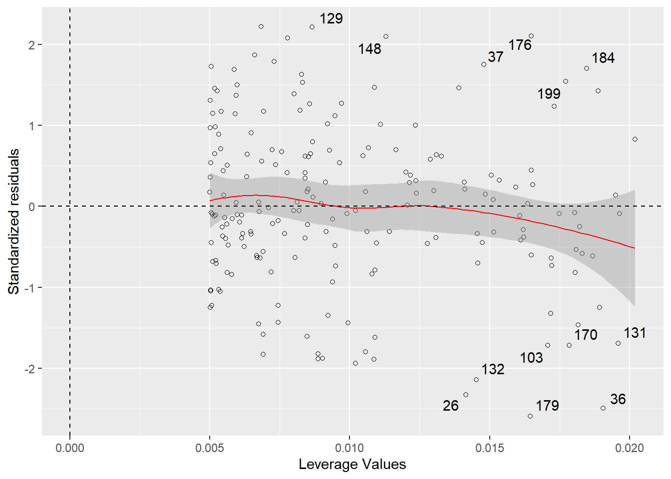
12.3.6 Cook‘s距离和杠杆值
Show the code
plot(lm_tv,6)