假设
正态性假设 (Normality) :
两组数据应来自正态分布的总体。对于大样本(通常 n > 30),由于中心极限定理,即使数据不完全符合正态分布,t 检验通常仍然稳健。
方差齐性假设 (Homoscedasticity) :
两组数据的方差应该相等。如果方差不相等,需使用 Welch’s t-test,它不假设方差齐性。
独立性假设 (Independence) :
样本中的观测应相互独立,一个观测的值不应影响另一个观测的值。
t检验类型
单样本t检验 (One-sample t-test): 用于比较单个样本的均值与已知的总体均值之间的差异。
独立样本t检验 (Independent samples t-test): 用于比较两个独立样本的均值差异。
配对样本t检验 (Paired samples t-test): 用于比较同一组受试者在两个不同条件下的均值差异。
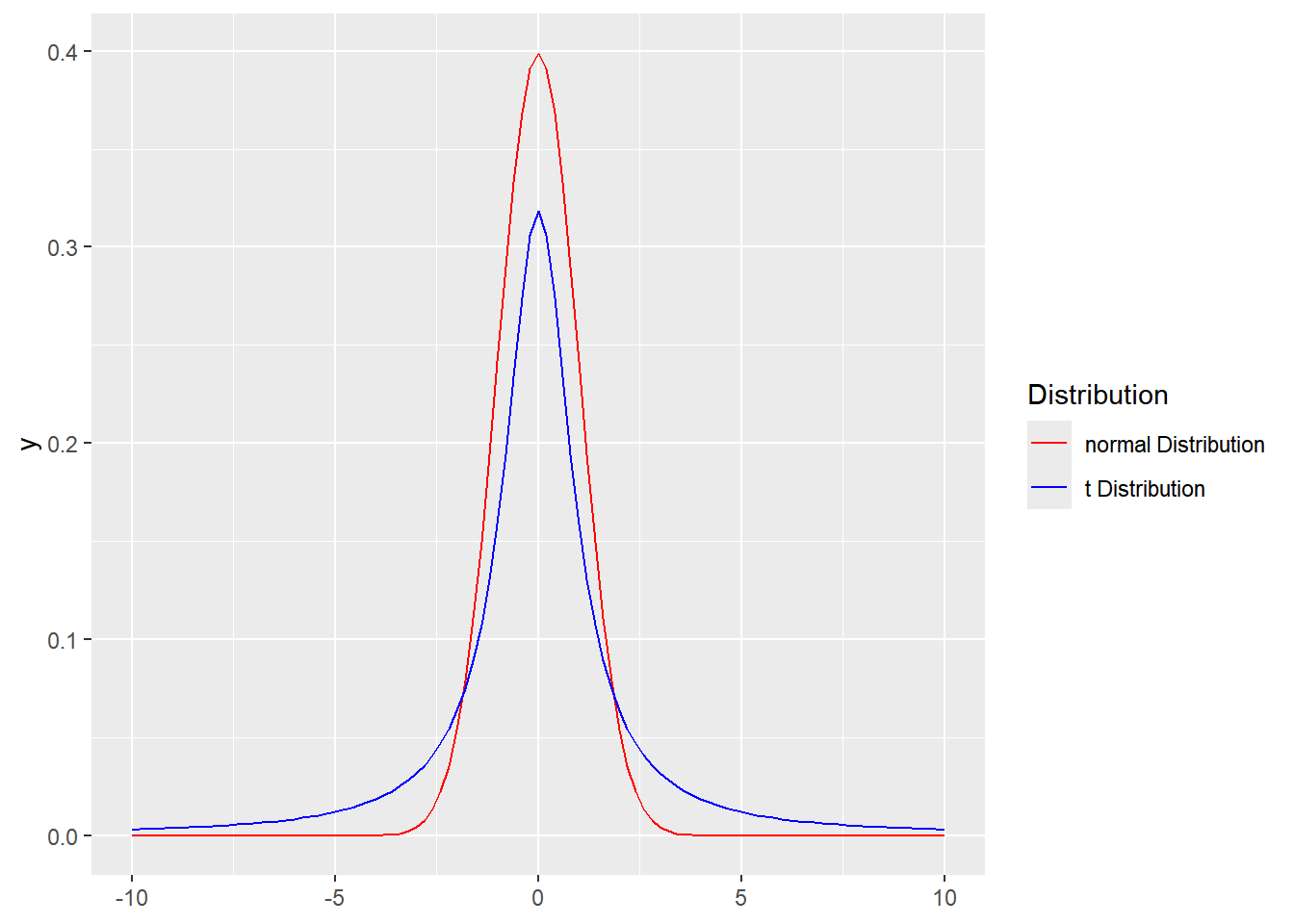
Show the code library ( tidyverse ) ggplot ( ) + xlim ( - 10 ,10 ) + geom_function ( mapping = aes ( color= "normal Distribution" ) ,
fun = dnorm , args = list ( mean = 0 , sd = 1 ) ,
) +
geom_function ( mapping = aes ( color= "t Distribution" ) ,
fun = dt , args = list ( df = 1 ,ncp= 0 ) ,
) +
scale_color_manual ( values = c ( "normal Distribution" = "red" ,
"t Distribution" = "blue" ) ) +
labs ( color = "Distribution" )
t 检验(Student‘s t test),主要用于小样本(n<30),标准差未知的正态分布总体。在进行t检验之前,可以先通过正态性检验 shapiro.test()
数据来源
2017.临床研究中的统计分析和图形表达实例详解 第2版
单样本 t 检验
在数据符合正态分布的前提下使用单样本t-test来比较一组样本的均值和已知(理论/总体)均值,所谓的已知均值能来自于之前的实验数据或者理论值。根据研究问题(原假设)的不同又分为双尾(不等)和单尾检验(大于或者小于)
\[t=\frac{\bar X-\mu_0}{S /\sqrt n} \sim t(\nu=n-1) \]
它是一种参数检验,用于检验样本均值是否可以合理地为总体均值或特定值。
Show the code Hb <- c ( 11.3 ,15.0 ,15.0 ,13.5 ,12.8 ,10.0 ,11.0 ,12.0 ,13.0 ,14.0 ) shapiro.test ( Hb ) #> #> Shapiro-Wilk normality test #> #> data: Hb #> W = 0.95907, p-value = 0.7752 t.test ( Hb , mu= 14.02 ) #> #> One Sample t-test #> #> data: Hb #> t = -2.3623, df = 9, p-value = 0.04244 #> alternative hypothesis: true mean is not equal to 14.02 #> 95 percent confidence interval: #> 11.55342 13.96658 #> sample estimates: #> mean of x #> 12.76
Show the code t_test_two_sided <- function ( data ,mu ,level = 0.95 ,... ) {
bar_X <- mean ( data ,na.rm = T )
sd <- sd ( data , na.rm = T )
n = length ( data )
se = sd / sqrt ( n )
t_statistic <- ( bar_X - mu ) / se
p_value <- 2 * ( 1 - pt ( abs ( t_statistic ) ,df= n - 1 ) )
t_critical <- qt ( ( 1 - ( 1 - level ) / 2 ) ,df = n - 1 )
CI_lower <- bar_X - t_critical * se
CI_upper <- bar_X + t_critical * se
CI <- paste0 ( level * 100 ,"% confidence interval: " ,"[" ,CI_lower ,"," ,CI_upper ,"]" ,sep = "" )
output <- data.frame (
均值= bar_X ,
标准差= sd ,
标准误= se ,
t= t_statistic ,
df= n - 1 ,
p_value= p_value ,
CI= CI
)
return ( output )
} t_test_two_sided ( Hb , mu= 14.02 ) #> 均值 标准差 标准误 t df p_value #> 1 12.76 1.68668 0.533375 -2.362315 9 0.04244005 #> CI #> 1 95% confidence interval: [11.5534219269741,13.9665780730259]
配对样本t检验
\[
H_0:\mu_{\bar d}=0
\] \[
t=\frac{\bar d- \mu_{\bar d}}{S_d /\sqrt n} \sim t(\nu)
\] 其中\(d= X_2-X_1,\mu_{\bar d}=0\) 。
Show the code df <- data.frame ( before = c ( 36 ,46 ,53 ,57 ,65 ,60 ,42 ,45 ,25 ,55 ,51 ,59 ) ,
after = c ( 45 ,64 ,66 ,57 ,70 ,55 ,70 ,45 ,50 ,80 ,60 ,60 )
) shapiro.test ( df $ before ) #> #> Shapiro-Wilk normality test #> #> data: df$before #> W = 0.95141, p-value = 0.6576 shapiro.test ( df $ after ) #> #> Shapiro-Wilk normality test #> #> data: df$after #> W = 0.96659, p-value = 0.872 t.test ( df $ after ,df $ before ,paired = TRUE ) #> #> Paired t-test #> #> data: df$after and df$before #> t = 3.3053, df = 11, p-value = 0.007011 #> alternative hypothesis: true mean difference is not equal to 0 #> 95 percent confidence interval: #> 3.563879 17.769455 #> sample estimates: #> mean difference #> 10.66667
独立样本的均值差异
方差齐性——F检验
\[H_0:\frac{\sigma_1^2}{\sigma_2^2}=1\]
\[
F=\frac{\frac {(n_1-1)S_1^2}{\sigma_1^2}/(n_1-1)}{\frac {(n_2-1)S_2^2}{\sigma_2^2}/(n_2-1)}=(\frac{S_1^2}{S_2^2})(\frac{\sigma_2^2}{\sigma_1^2})=\frac{S_1^2}{S_2^2}\sim F(\nu_1,\nu_2),\nu_1=n_1-1,\nu_2=n_2-1
\]
Show the code test_group = c ( 10.2 , 8.9 , 10.1 , 9.2 , - 0.8 , 10.6 , 6.5 , 11.2 , 9.3 , 8.0 , 10.7 , 9.5 , 12.7 , 14.4 , 11.9 ) healthy_group = c ( 5.0 , 6.7 , - 1.4 , 4.0 , 7.1 , - 0.6 , 2.8 , 4.3 , 3.7 , 5.8 , 4.6 , 6.0 , 4.1 , 5.1 , 4.7 ) # 检验两个样本的方差是否相等 var.test ( test_group , healthy_group ) #> #> F test to compare two variances #> #> data: test_group and healthy_group #> F = 2.0812, num df = 14, denom df = 14, p-value = 0.1827 #> alternative hypothesis: true ratio of variances is not equal to 1 #> 95 percent confidence interval: #> 0.6987342 6.1991582 #> sample estimates: #> ratio of variances #> 2.081241 # car::leveneTest()
方差齐——t检验
\[H_0:\mu_1-\mu_2=0\]
\[
t=\frac{(\bar X_1-\bar X_2)-(\mu_1-\mu_2)}{S_{\bar X_1-\bar X_2}}=\frac{\bar X_1-\bar X_2}{S_C\sqrt{(\frac{1}{n_1}+\frac{1}{n_2})}}
\]
其中,\(S_c^2=\frac{(n_1-1)S_1^2+(n_2-1)S_2^2}{n_1+n_2-2}\)
Show the code # 方差齐 t.test ( test_group , healthy_group , conf.level = 0.95 , var.equal = TRUE ) #> #> Two Sample t-test #> #> data: test_group and healthy_group #> t = 4.9875, df = 28, p-value = 2.869e-05 #> alternative hypothesis: true difference in means is not equal to 0 #> 95 percent confidence interval: #> 3.162555 7.570779 #> sample estimates: #> mean of x mean of y #> 9.493333 4.126667
方差不齐—— Approximation t 检验
\[H_0:\mu_1-\mu_2=0\]
\[
t'=\frac{(\bar X_1-\bar X_2)-(\mu_1-\mu_2)}{\sqrt{\frac{S_1^2}{n_1}+\frac{S_2^2}{n_2}}}=\frac{\bar X_1-\bar X_2}{\sqrt{\frac{S_1^2}{n_1}+\frac{S_2^2}{n_2}}}\sim t(\nu ')
\]
Welch /Satterthwaite t-test
强调自由度
\[
v'=\frac{(\frac{S_1^2}{n_1}+\frac{S_2^2}{n_2})^2}{\frac{(\frac{S_1^2}{n_1})^2}{n_1-1}+\frac{(\frac{S_2^2}{n_2})^2}{n_2-1}}(舍入到最近整数)
\]
Show the code # 假设方差不齐,使用Welch t检验 t.test ( test_group , healthy_group , conf.level = 0.95 ) #> #> Welch Two Sample t-test #> #> data: test_group and healthy_group #> t = 4.9875, df = 24.93, p-value = 3.878e-05 #> alternative hypothesis: true difference in means is not equal to 0 #> 95 percent confidence interval: #> 3.150262 7.583071 #> sample estimates: #> mean of x mean of y #> 9.493333 4.126667