3 相关性

Modified

January 9, 2026

https://corrr.tidymodels.org/articles/using-corrr.html

https://easystats.github.io/correlation/

相关性：判断两个变量之间的相关关系强度和方向，无论是否独立。

Show the code

library(easystats)

3.1 连续变量

如果两个连续变量不相互独立时，使用协方差（covariance）来描述两个变量的关系。

协方差（或相关系数）为零，不相关，说明不存在线性关系，但可能存在非线性关系。

Show the code

df <- iris[1:4]

# 协方差矩阵
cov(df)    
#>              Sepal.Length Sepal.Width Petal.Length Petal.Width
#> Sepal.Length    0.6856935  -0.0424340    1.2743154   0.5162707
#> Sepal.Width    -0.0424340   0.1899794   -0.3296564  -0.1216394
#> Petal.Length    1.2743154  -0.3296564    3.1162779   1.2956094
#> Petal.Width     0.5162707  -0.1216394    1.2956094   0.5810063

3.1.0.1 相关系数

相关系数的取值范围： \([-1,1]\)

\[ r(X,Y)=\frac {\sum_{i=1}^n (x_i-\bar x)(y_i-\bar y)}{\sqrt{\sum_{i=1}^n (x_i-\bar x)^2 \sum_{i=1}^n (y_i-\bar y)^2}} \]

Show the code

# Pearson's 积差相关系数 一般要求两个连续变量都服从正态分布
correlation(df,method = "pearson",p_adjust = "holm")
#> # Correlation Matrix (pearson-method)
#> 
#> Parameter1   |   Parameter2 |     r |         95% CI | t(148) |         p
#> -------------------------------------------------------------------------
#> Sepal.Length |  Sepal.Width | -0.12 | [-0.27,  0.04] |  -1.44 | 0.152    
#> Sepal.Length | Petal.Length |  0.87 | [ 0.83,  0.91] |  21.65 | < .001***
#> Sepal.Length |  Petal.Width |  0.82 | [ 0.76,  0.86] |  17.30 | < .001***
#> Sepal.Width  | Petal.Length | -0.43 | [-0.55, -0.29] |  -5.77 | < .001***
#> Sepal.Width  |  Petal.Width | -0.37 | [-0.50, -0.22] |  -4.79 | < .001***
#> Petal.Length |  Petal.Width |  0.96 | [ 0.95,  0.97] |  43.39 | < .001***
#> 
#> p-value adjustment method: Holm (1979)
#> Observations: 150

# Spearman's rank rho相关系数  　　非参数
correlation(df,method = "spearman",p_adjust = "holm")
#> # Correlation Matrix (spearman-method)
#> 
#> Parameter1   |   Parameter2 |   rho |         95% CI |        S |         p
#> ---------------------------------------------------------------------------
#> Sepal.Length |  Sepal.Width | -0.17 | [-0.32,  0.00] | 6.56e+05 | 0.041*   
#> Sepal.Length | Petal.Length |  0.88 | [ 0.84,  0.91] | 66429.35 | < .001***
#> Sepal.Length |  Petal.Width |  0.83 | [ 0.78,  0.88] | 93208.42 | < .001***
#> Sepal.Width  | Petal.Length | -0.31 | [-0.45, -0.15] | 7.37e+05 | < .001***
#> Sepal.Width  |  Petal.Width | -0.29 | [-0.43, -0.13] | 7.25e+05 | < .001***
#> Petal.Length |  Petal.Width |  0.94 | [ 0.91,  0.95] | 35060.85 | < .001***
#> 
#> p-value adjustment method: Holm (1979)
#> Observations: 150

# Kendall's rank tau相关系数  　　非参数
correlation(df,method = "kendall",p_adjust = "holm")
#> # Correlation Matrix (kendall-method)
#> 
#> Parameter1   |   Parameter2 |   tau |         95% CI |     z |         p
#> ------------------------------------------------------------------------
#> Sepal.Length |  Sepal.Width | -0.08 | [-0.18,  0.03] | -1.33 | 0.183    
#> Sepal.Length | Petal.Length |  0.72 | [ 0.66,  0.77] | 12.65 | < .001***
#> Sepal.Length |  Petal.Width |  0.66 | [ 0.59,  0.71] | 11.34 | < .001***
#> Sepal.Width  | Petal.Length | -0.19 | [-0.29, -0.08] | -3.22 | 0.004**  
#> Sepal.Width  |  Petal.Width | -0.16 | [-0.26, -0.05] | -2.67 | 0.015*   
#> Petal.Length |  Petal.Width |  0.81 | [ 0.77,  0.84] | 13.97 | < .001***
#> 
#> p-value adjustment method: Holm (1979)
#> Observations: 150

3.1.0.2 相关图（correlogram）

Show the code

library(see)

correlation(df,method = "pearson",p_adjust = "holm") |>
  summary(redundant = TRUE) |>  
  plot()

3.1.0.3 显著性检验

　　零假设为变量之间不相关（即两个总体的相关系数为 0 ）。函数 cor.test( ) 可用于对相关系数进行显著性检验。

统计量

\[ t=\frac{r\sqrt{n-2}}{\sqrt{1-r^2}} \]

Show the code

cor_test(df, "Sepal.Length", "Sepal.Width")
#> Parameter1   |  Parameter2 |     r |        95% CI | t(148) |     p
#> -------------------------------------------------------------------
#> Sepal.Length | Sepal.Width | -0.12 | [-0.27, 0.04] |  -1.44 | 0.152
#> 
#> Observations: 150

psych包corr.test() 计算相关系数矩阵和显著性检验

Show the code

psych::corr.test(df)
#> Call:psych::corr.test(x = df)
#> Correlation matrix 
#>              Sepal.Length Sepal.Width Petal.Length Petal.Width
#> Sepal.Length         1.00       -0.12         0.87        0.82
#> Sepal.Width         -0.12        1.00        -0.43       -0.37
#> Petal.Length         0.87       -0.43         1.00        0.96
#> Petal.Width          0.82       -0.37         0.96        1.00
#> Sample Size 
#> [1] 150
#> Probability values (Entries above the diagonal are adjusted for multiple tests.) 
#>              Sepal.Length Sepal.Width Petal.Length Petal.Width
#> Sepal.Length         0.00        0.15            0           0
#> Sepal.Width          0.15        0.00            0           0
#> Petal.Length         0.00        0.00            0           0
#> Petal.Width          0.00        0.00            0           0
#> 
#>  To see confidence intervals of the correlations, print with the short=FALSE option

print(psych::corr.test(df), short = FALSE)
#> Call:psych::corr.test(x = df)
#> Correlation matrix 
#>              Sepal.Length Sepal.Width Petal.Length Petal.Width
#> Sepal.Length         1.00       -0.12         0.87        0.82
#> Sepal.Width         -0.12        1.00        -0.43       -0.37
#> Petal.Length         0.87       -0.43         1.00        0.96
#> Petal.Width          0.82       -0.37         0.96        1.00
#> Sample Size 
#> [1] 150
#> Probability values (Entries above the diagonal are adjusted for multiple tests.) 
#>              Sepal.Length Sepal.Width Petal.Length Petal.Width
#> Sepal.Length         0.00        0.15            0           0
#> Sepal.Width          0.15        0.00            0           0
#> Petal.Length         0.00        0.00            0           0
#> Petal.Width          0.00        0.00            0           0
#> 
#>  Confidence intervals based upon normal theory.  To get bootstrapped values, try cor.ci
#>             raw.lower raw.r raw.upper raw.p lower.adj upper.adj
#> Spl.L-Spl.W     -0.27 -0.12      0.04  0.15     -0.27      0.04
#> Spl.L-Ptl.L      0.83  0.87      0.91  0.00      0.81      0.91
#> Spl.L-Ptl.W      0.76  0.82      0.86  0.00      0.74      0.88
#> Spl.W-Ptl.L     -0.55 -0.43     -0.29  0.00     -0.58     -0.25
#> Spl.W-Ptl.W     -0.50 -0.37     -0.22  0.00     -0.51     -0.20
#> Ptl.L-Ptl.W      0.95  0.96      0.97  0.00      0.94      0.98

3.2 分类变量

　　如果独立性检验的结果表明两个变量之间不独立，那么如何量化它们之间相关性的强弱?

3.2.1 列联系数、Phi 系数和 Cramer’s V 系数

vcd 包里的函数 assocstats( )可以用来计算列联表的 Phi 系数、列联系数和 Cramer’s V 系数。其中， Phi 系数只适用于四格表。　　

Show the code

library(vcd)
mytable <- table(Arthritis$Sex, Arthritis$Treatment)
assocstats(mytable)
#>                      X^2 df P(> X^2)
#> Likelihood Ratio 0.73748  1  0.39047
#> Pearson          0.73653  1  0.39078
#> 
#> Phi-Coefficient   : 0.094 
#> Contingency Coeff.: 0.093 
#> Cramer's V        : 0.094

3.2.2 Kappa 统计量

对于配对列联表，可以计算一致性指标 Kappa 统计量。 epiDisplay 包里的函数 kap( )可以用于计算一致性的比例以及 Kappa 统计量的值　　　　

Show the code

my.matrix <- matrix(c(11, 2, 12, 33), nrow = 2)
sum(my.matrix)
#> [1] 58
vcd::Kappa(my.matrix)
#>            value    ASE     z Pr(>|z|)
#> Unweighted 0.455 0.1153 3.945 7.97e-05
#> Weighted   0.455 0.1153 3.945 7.97e-05
epiDisplay::kap(my.matrix)
#> 
#>  Table for calculation of kappa
#>    A  B
#> A 11 12
#> B  2 33
#> 
#> Observed agreement = 75.86 % 
#> Expected agreement = 55.71 % 
#> Kappa = 0.455 
#> Standard error = 0.121 , Z = 3.762 , P value = < 0.001 
#>

　　共 58 个对象，每一对象用两种检测方法检测，其中11 个对象的两种检测结果都为阳性， 33 个对象的两种检测结果都是阴性，所以总一致性为 (11 + 33)/58 ≈ 75.86% 。

Show the code

chisq.test(my.matrix)$expected
#>          [,1]     [,2]
#> [1,] 5.155172 17.84483
#> [2,] 7.844828 27.15517

　为了解释期望一致性和 Kappa 值的含义，先计算各个单元格的期望频数。对角线上的这两个单元格对应的期望频数分别约为5.155172 和27.15517 ，因此期望一致性为 (5.155172+27.15517)/58≈ 55.71% 。期望一致性是假定两种方法的检测结果都是完全随机的情况下的一致性。也就是说，即使两种检测方法都毫无作用，平均也能达到 55.71% 的一致性。 Kappa 统计量是超出随机的一致性的部分占最大可能超出随机的一致性的比例。在本例中，前者为 75.86% − 55.71% ，后者为 100% − 55.71% 。因此， Kappa 值为 (75.86 - 55.71)/(100 - 55.71) ≈ 0.455

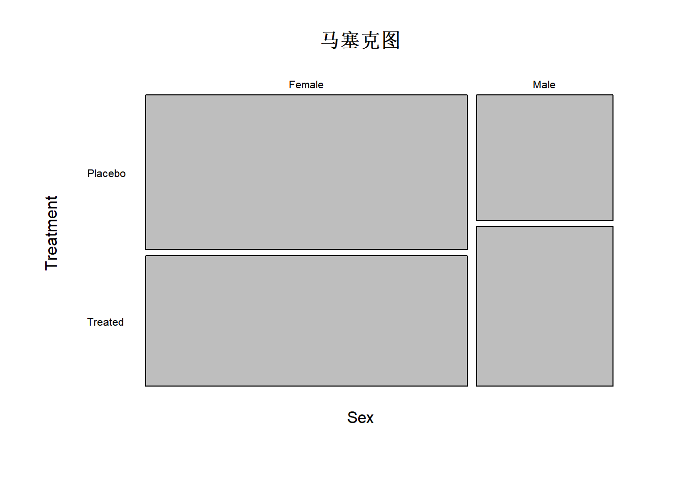
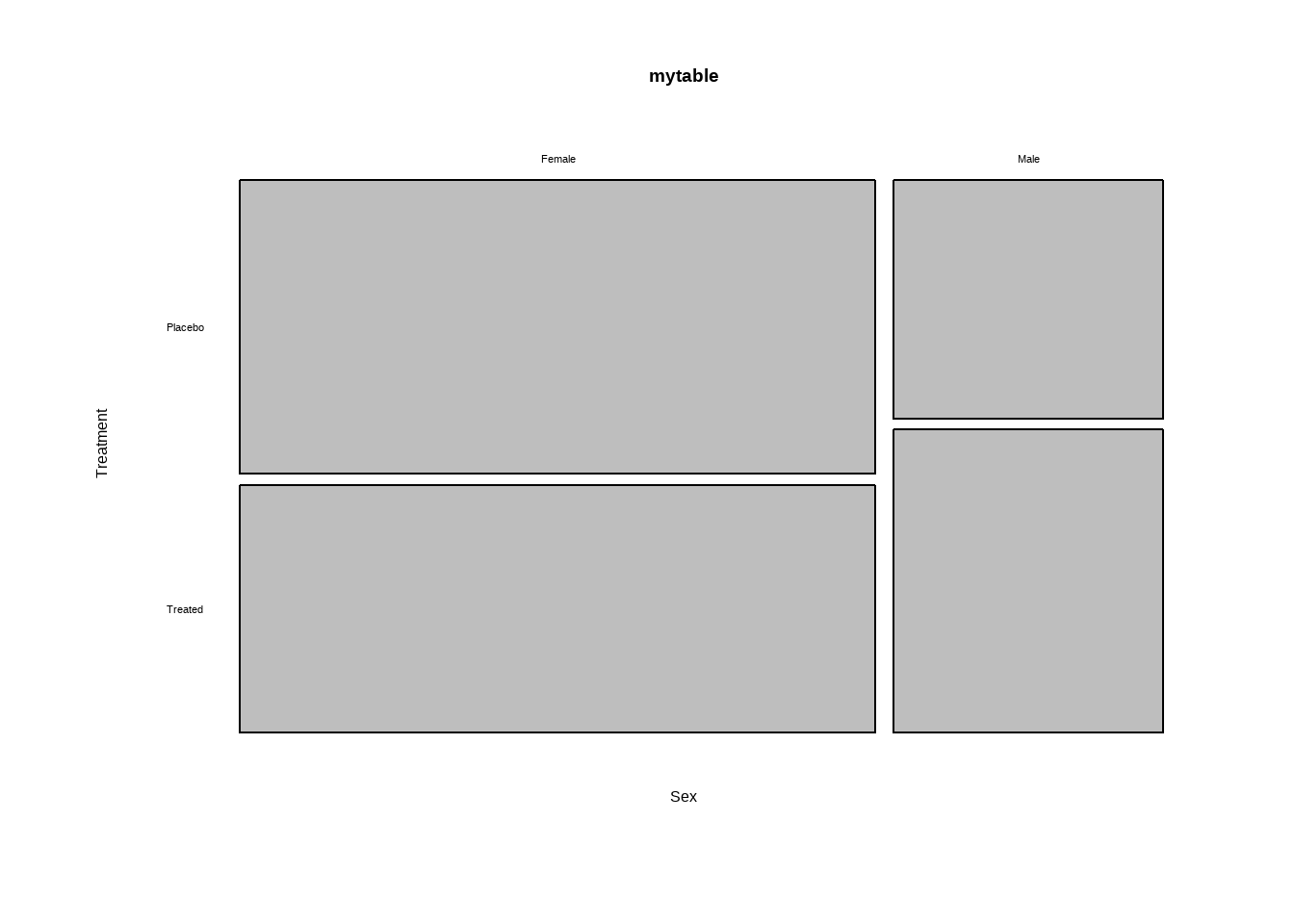
3.2.3 马赛克图

　　马赛克图中的矩形面积正比于多维列联表中单元格的频率　　

Show the code

mosaicplot(mytable,main ="马塞克图" ,
           xlab ="Sex",ylab =  "Treatment",las = 1)