# 医学统计学 人卫版 第7版SBP<-read_tsv("data/麻醉诱导时相.tsv")SBP#> # A tibble: 15 × 7#> id group t0 t1 t2 t3 t4#> <dbl> <chr> <dbl> <dbl> <dbl> <dbl> <dbl>#> 1 1 A 120 108 112 120 117#> 2 2 A 118 109 115 126 123#> 3 3 A 119 112 119 124 118#> 4 4 A 121 112 119 126 120#> 5 5 A 127 121 127 133 126#> 6 6 B 121 120 118 131 137#> 7 7 B 122 121 119 129 133#> 8 8 B 128 129 126 135 142#> 9 9 B 117 115 111 123 131#> 10 10 B 118 114 116 123 133#> 11 11 C 131 119 118 135 129#> 12 12 C 129 128 121 148 132#> 13 13 C 123 123 120 143 136#> 14 14 C 123 121 116 145 126#> 15 15 C 125 124 118 142 130
Show the code
SBP_long<-SBP|>pivot_longer(cols =starts_with("t"), names_to ="time", values_to ="SBP")|>mutate( id=factor(id), group=factor(group), time=factor(time))SBP_long%>%head()#> # A tibble: 6 × 4#> id group time SBP#> <fct> <fct> <fct> <dbl>#> 1 1 A t0 120#> 2 1 A t1 108#> 3 1 A t2 112#> 4 1 A t3 120#> 5 1 A t4 117#> 6 2 A t0 118
Show the code
# 正态性检验library(rstatix)SBP_long%>%group_by(time,group)%>%shapiro_test(SBP)#> # A tibble: 15 × 5#> group time variable statistic p#> <fct> <fct> <chr> <dbl> <dbl>#> 1 A t0 SBP 0.836 0.154#> 2 B t0 SBP 0.916 0.503#> 3 C t0 SBP 0.867 0.254#> 4 A t1 SBP 0.834 0.148#> 5 B t1 SBP 0.913 0.485#> 6 C t1 SBP 0.978 0.921#> 7 A t2 SBP 0.940 0.666#> 8 B t2 SBP 0.969 0.869#> 9 C t2 SBP 0.953 0.758#> 10 A t3 SBP 0.937 0.647#> 11 B t3 SBP 0.902 0.421#> 12 C t3 SBP 0.941 0.672#> 13 A t4 SBP 0.943 0.687#> 14 B t4 SBP 0.892 0.367#> 15 C t4 SBP 0.984 0.955
8.3.2.1nlme::lme()
Show the code
# 第一种方法library(nlme)SBP_lme<-lme(SBP~group*time, random =~1|id/time, data =SBP_long)# summary(SBP_lme)anova(SBP_lme)#> numDF denDF F-value p-value#> (Intercept) 1 48 14649.223 <.0001#> group 2 12 5.783 0.0174#> time 4 48 106.558 <.0001#> group:time 8 48 19.101 <.0001# 看不到球形检验# 事后检验 成对比较library(emmeans)# 如果交互效应不显著## 时间点事后检验SBP_long%>%pairwise_t_test(SBP~time, p.adjust.method ="none", detailed =TRUE)#> # A tibble: 10 × 10#> .y. group1 group2 n1 n2 p method p.adj p.signif p.adj.signif#> * <chr> <chr> <chr> <int> <int> <dbl> <chr> <dbl> <chr> <chr> #> 1 SBP t0 t1 15 15 6.81e-2 T-test 6.81e-2 ns ns #> 2 SBP t0 t2 15 15 6.41e-2 T-test 6.41e-2 ns ns #> 3 SBP t1 t2 15 15 9.78e-1 T-test 9.78e-1 ns ns #> 4 SBP t0 t3 15 15 1.78e-4 T-test 1.78e-4 *** *** #> 5 SBP t1 t3 15 15 1.67e-7 T-test 1.67e-7 **** **** #> 6 SBP t2 t3 15 15 1.49e-7 T-test 1.49e-7 **** **** #> 7 SBP t0 t4 15 15 1.28e-2 T-test 1.28e-2 * * #> 8 SBP t1 t4 15 15 3.68e-5 T-test 3.68e-5 **** **** #> 9 SBP t2 t4 15 15 3.32e-5 T-test 3.32e-5 **** **** #> 10 SBP t3 t4 15 15 1.65e-1 T-test 1.65e-1 ns nsemmeans(SBP_lme,pairwise~time, adjust ="none")#> $emmeans#> time emmean SE df lower.CL upper.CL#> t0 123 1.16 12 120 125#> t1 118 1.16 12 116 121#> t2 118 1.16 12 116 121#> t3 132 1.16 12 130 135#> t4 129 1.16 12 126 131#> #> Results are averaged over the levels of: group #> Degrees-of-freedom method: containment #> Confidence level used: 0.95 #> #> $contrasts#> contrast estimate SE df t.ratio p.value#> t0 - t1 4.4000 0.855 48 5.147 <.0001#> t0 - t2 4.4667 0.855 48 5.225 <.0001#> t0 - t3 -9.4000 0.855 48 -10.995 <.0001#> t0 - t4 -6.0667 0.855 48 -7.096 <.0001#> t1 - t2 0.0667 0.855 48 0.078 0.9382#> t1 - t3 -13.8000 0.855 48 -16.142 <.0001#> t1 - t4 -10.4667 0.855 48 -12.243 <.0001#> t2 - t3 -13.8667 0.855 48 -16.220 <.0001#> t2 - t4 -10.5333 0.855 48 -12.321 <.0001#> t3 - t4 3.3333 0.855 48 3.899 0.0003#> #> Results are averaged over the levels of: group #> Degrees-of-freedom method: containment## 组间事后检验emmeans(SBP_lme,pairwise~group, adjust ="none")# 与spss一样#> $emmeans#> group emmean SE df lower.CL upper.CL#> A 120 1.78 14 116 123#> B 124 1.78 12 121 128#> C 128 1.78 12 124 132#> #> Results are averaged over the levels of: time #> Degrees-of-freedom method: containment #> Confidence level used: 0.95 #> #> $contrasts#> contrast estimate SE df t.ratio p.value#> A - B -4.80 2.51 12 -1.911 0.0802#> A - C -8.52 2.51 12 -3.392 0.0054#> B - C -3.72 2.51 12 -1.481 0.1644#> #> Results are averaged over the levels of: time #> Degrees-of-freedom method: containment# 此处交互效应显著# 1. 简单组别效应 与SPSS一样SBP_long%>%group_by(time)%>%anova_test(SBP~group)#> # A tibble: 5 × 8#> time Effect DFn DFd F p `p<.05` ges#> * <fct> <chr> <dbl> <dbl> <dbl> <dbl> <chr> <dbl>#> 1 t0 group 2 12 2.93 0.092 "" 0.328#> 2 t1 group 2 12 6.03 0.015 "*" 0.501#> 3 t2 group 2 12 0.022 0.979 "" 0.004#> 4 t3 group 2 12 17.0 0.000312 "*" 0.74 #> 5 t4 group 2 12 17.4 0.000286 "*" 0.743# 2. 各时间点处理组成对比较 用的是未调整的p值,无法观察到标准误SBP_long%>%group_by(time)%>%pairwise_t_test(SBP~group, p.adjust.method ="bonferroni", detailed =TRUE)#> # A tibble: 15 × 11#> time .y. group1 group2 n1 n2 p method p.adj p.signif#> * <fct> <chr> <chr> <chr> <int> <int> <dbl> <chr> <dbl> <chr> #> 1 t0 SBP A B 5 5 0.936 T-test 1 ns #> 2 t0 SBP A C 5 5 0.0539 T-test 0.162 ns #> 3 t0 SBP B C 5 5 0.0623 T-test 0.187 ns #> 4 t1 SBP A B 5 5 0.0358 T-test 0.107 * #> 5 t1 SBP A C 5 5 0.00541 T-test 0.0162 ** #> 6 t1 SBP B C 5 5 0.327 T-test 0.981 ns #> 7 t2 SBP A B 5 5 0.894 T-test 1 ns #> 8 t2 SBP A C 5 5 0.947 T-test 1 ns #> 9 t2 SBP B C 5 5 0.842 T-test 1 ns #> 10 t3 SBP A B 5 5 0.456 T-test 1 ns #> 11 t3 SBP A C 5 5 0.000161 T-test 0.000483 *** #> 12 t3 SBP B C 5 5 0.000585 T-test 0.00175 *** #> 13 t4 SBP A B 5 5 0.0000887 T-test 0.000266 **** #> 14 t4 SBP A C 5 5 0.00201 T-test 0.00602 ** #> 15 t4 SBP B C 5 5 0.0901 T-test 0.27 ns #> # ℹ 1 more variable: p.adj.signif <chr>
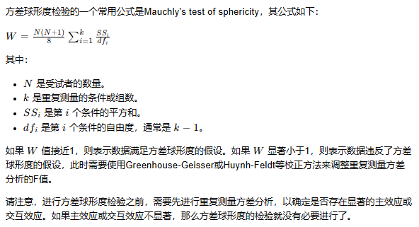
8.3.2.2rstatix::anova_test() 看球形检验 W统计量
Show the code
library(rstatix)aov_SBP<-anova_test(data =SBP_long, dv =SBP, wid =id, within =time, between =group, type ="3")aov_SBP#> ANOVA Table (type III tests)#> #> $ANOVA#> Effect DFn DFd F p p<.05 ges#> 1 group 2 12 5.783 1.70e-02 * 0.430#> 2 time 4 48 106.558 3.02e-23 * 0.659#> 3 group:time 8 48 19.101 1.62e-12 * 0.409#> #> $`Mauchly's Test for Sphericity`#> Effect W p p<.05#> 1 time 0.293 0.178 #> 2 group:time 0.293 0.178 #> #> $`Sphericity Corrections`#> Effect GGe DF[GG] p[GG] p[GG]<.05 HFe DF[HF] p[HF]#> 1 time 0.679 2.71, 32.58 1.87e-16 * 0.896 3.59, 43.03 4.65e-21#> 2 group:time 0.679 5.43, 32.58 4.26e-09 * 0.896 7.17, 43.03 2.04e-11#> p[HF]<.05#> 1 *#> 2 *# 进行事后检验,若交互效应不显著SBP_long%>%group_by(time)%>%pairwise_t_test(SBP~group, p.adjust.method ="bonferroni", detailed =TRUE)#> # A tibble: 15 × 11#> time .y. group1 group2 n1 n2 p method p.adj p.signif#> * <fct> <chr> <chr> <chr> <int> <int> <dbl> <chr> <dbl> <chr> #> 1 t0 SBP A B 5 5 0.936 T-test 1 ns #> 2 t0 SBP A C 5 5 0.0539 T-test 0.162 ns #> 3 t0 SBP B C 5 5 0.0623 T-test 0.187 ns #> 4 t1 SBP A B 5 5 0.0358 T-test 0.107 * #> 5 t1 SBP A C 5 5 0.00541 T-test 0.0162 ** #> 6 t1 SBP B C 5 5 0.327 T-test 0.981 ns #> 7 t2 SBP A B 5 5 0.894 T-test 1 ns #> 8 t2 SBP A C 5 5 0.947 T-test 1 ns #> 9 t2 SBP B C 5 5 0.842 T-test 1 ns #> 10 t3 SBP A B 5 5 0.456 T-test 1 ns #> 11 t3 SBP A C 5 5 0.000161 T-test 0.000483 *** #> 12 t3 SBP B C 5 5 0.000585 T-test 0.00175 *** #> 13 t4 SBP A B 5 5 0.0000887 T-test 0.000266 **** #> 14 t4 SBP A C 5 5 0.00201 T-test 0.00602 ** #> 15 t4 SBP B C 5 5 0.0901 T-test 0.27 ns #> # ℹ 1 more variable: p.adj.signif <chr>
group__summary<-SBP_long|>group_by(group)|>summarise(n=n(),mean=mean(SBP),sum=sum(SBP))group__summary#> # A tibble: 3 × 4#> group n mean sum#> <fct> <int> <dbl> <dbl>#> 1 A 25 120. 2992#> 2 B 25 124. 3112#> 3 C 25 128. 3205
SS处理
\[
SS_{处理}= \sum_i^k n_k (\bar X_k - \bar X)^2
\]
其中,k为不同处理组的组数,nk 为第 k 处理组观测值的总数,\(\bar X_k\) 为第k 处理组观测值的均数,\(\bar X\) 是所有观测值的均值。